Fine-scale movement modeling based on tagging data

This tutorial illustrates the application of the momo package to model fine-scale movement based on tagging data.

Outline:

1. Prepare the data
2. Fit the model
3. Results
4. Advanced settings
5. Summary
6. References

The package is loaded into the R environment with:

library(momo)

This introductory tutorial uses a simulated data set included in the package: “skjepo”. We load it into the R environment with the command data(skjepo).

This command loads not only the main list object skjepo (of class momo.sim), which contains all required simulated data and can be used right away to fit the model, but also four individual data sets: skjepo.grid, skjepo.env, skjepo.ctags, and skjepo.atags. These data sets illustrate the typical structure of raw input data and demonstrate how the functions in the momo package can be used to convert them into the format required by the model as demonstrated in the next section.

Prepare the data

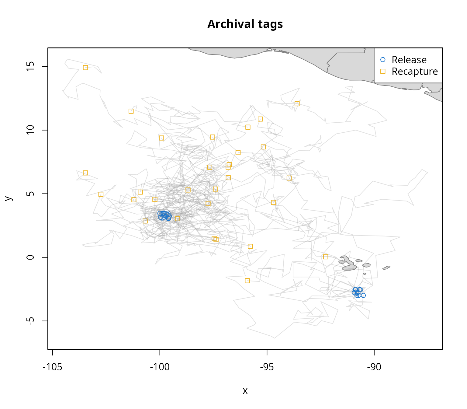
The package provides two main data sets: one with information on releases and recoveries of conventional tags, and another with track data from archival tags. These data sets can be prepared for analysis using the built-in functions prep.ctags and prep.atags. Both functions allow users to specify which columns contain the release and recapture times and locations, and automatically convert date fields to the required format. Additional features, such as a speed filter to flag implausible movements, are also available. For full details on how to use each function, refer to their respective help pages (e.g., help("prep.ctags")).

#> Removing 5 recaptured tags for which release time is after recapture time (t0 > t1).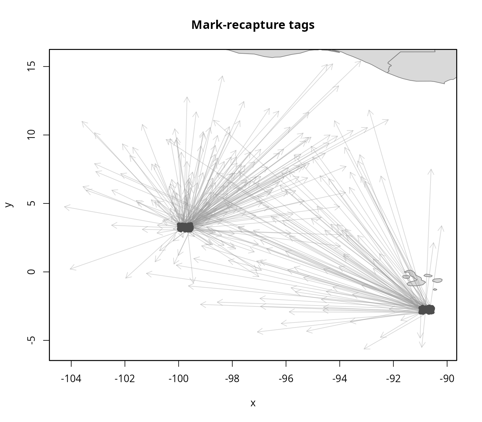

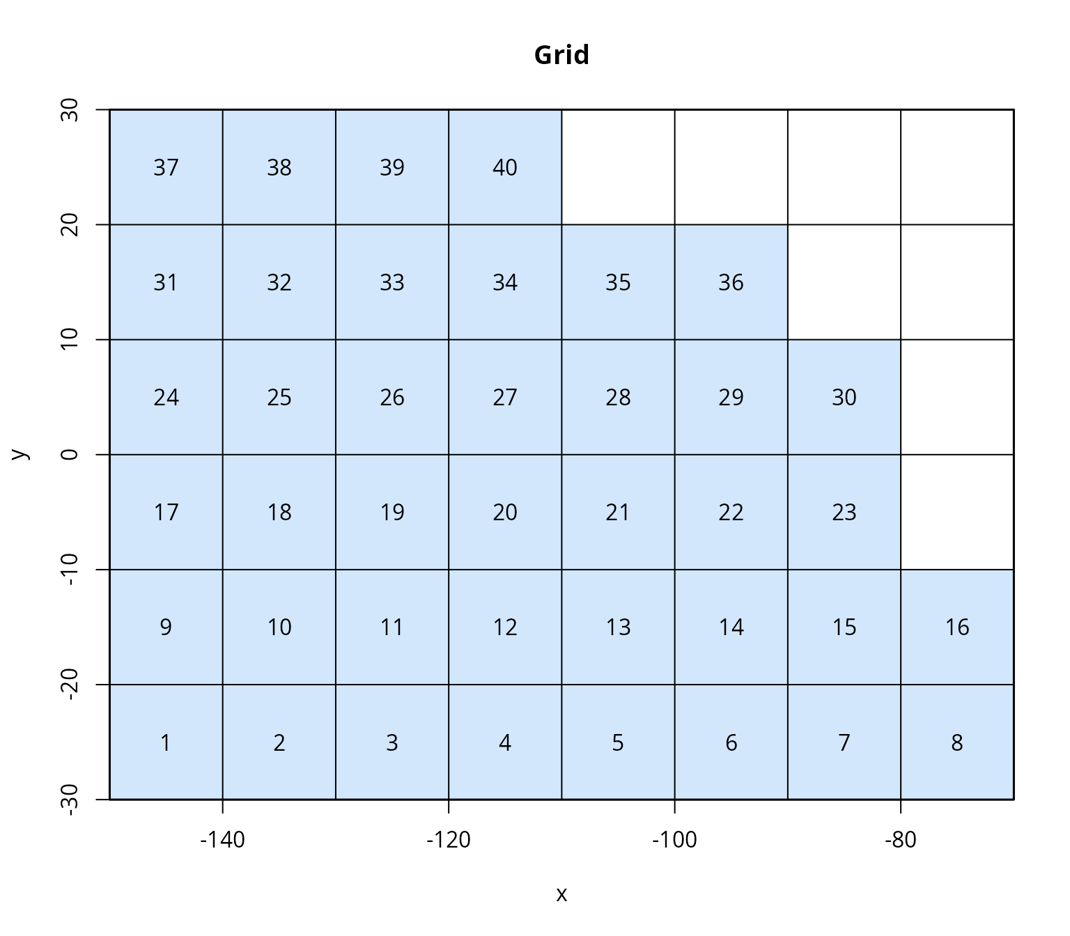
Based on the spatial extent of the tagging data, the next step is to define a spatial grid. While the Kalman filter approach does not require a grid for model fitting (Mildenberger, Maunder, and Nielsen in prep), using a grid enables spatial prediction, visualization, and analysis of estimated habitat preferences and movement rates. The create.grid function offers flexible functionality to define custom grids and to manually include or exclude specific grid cells as needed.

Since manual selection of grid cells is not feasible in this automated vignette, we use the grid provided in the skjepo data set, but modify it to create a coarser resolution:

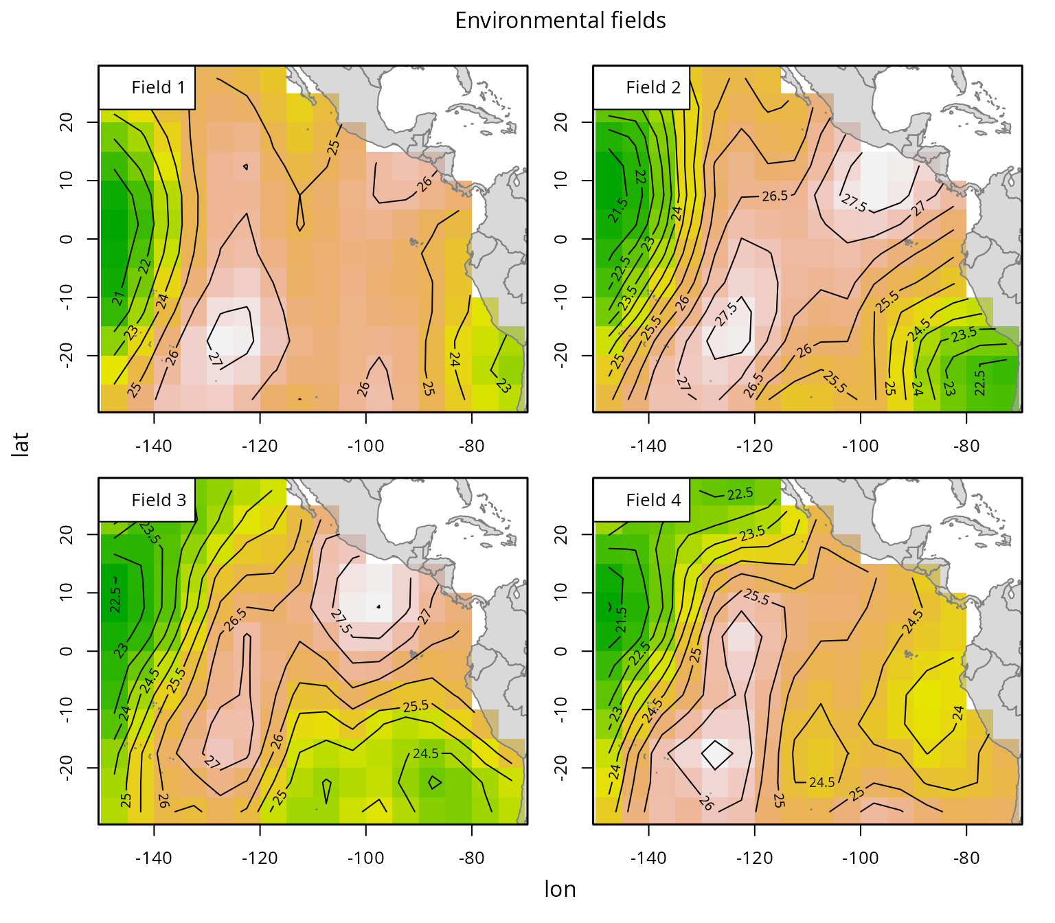
Another important component of momo is the environmental data, which characterizes the habitat preferences of the modeled species. The prep.env function formats this data into the structure required by the model:

To speed up the fitting process in this vignette, we use a subset of the available conventional tag data:

The individual data sets can then be combined into a single input object using the setup.momo.data function.

The def.conf function generates a list of default configuration settings, including flags that control which model functionalities are activated and how environmental fields are aligned with the model’s time steps. It is good practice to review this configuration list to ensure that the default settings align with the goals and structure of your analysis.

Similarly, the def.par function generates a list of default model parameters and their initial values. While users can adjust the initial values as needed, caution is required when modifying parameter dimensions. These dimensions must be consistent with the input data (e.g., the number of environmental fields) and the configuration settings (e.g., whether passive advection, taxis, or both are used).

With all necessary input data prepared, the model is now ready to be fitted using momo.

Fit the model

The model is fitted using the fit.momo function. Depending on the model’s complexity and the number of tags, this step may take several minutes. To reduce computation time, we disable the calculation of uncertainty estimates by setting do.sdreport = FALSE.

#> Building the model, that can take a few minutes.
#> Model built (0.49min). Minimizing neg. loglik.
#>   0:     1595143.9:  0.00000  0.00000 -4.60517 -4.60517
#>   1:     635104.70: -0.00109162 0.00103431 -3.80611 -4.00393
#>   2:     304398.49: -0.00321421 0.00304836 -3.65852 -3.01488
#>   3:     170499.70: -0.0452335 0.0429272 -3.57747 -2.01986
#>   4:     69216.328: -0.0488214 0.0463318 -2.68219 -1.57439
#>   5:     39735.044: -0.0693510 0.0658124 -1.74462 -1.92105
#>   6:     16219.655: -0.0717639 0.0681009 -0.957443 -1.30433
#>   7:     8947.6279: -0.0944541 0.0896236 0.0237874 -1.49461
#>   8:     5023.3234: -0.0783233 0.0743135 0.700975 -0.759138
#>   9:     3583.2798: -0.0822662 0.0780472  1.69448 -0.872793
#>  10:     3081.8592: -0.0855251 0.0811369  2.56455 -1.36571
#>  11:     3051.9565: -0.293328 0.277865  2.56205 -2.32389
#>  12:     3044.8443: -0.848239 0.802450  3.03697 -2.76131
#>  13:     3012.0243: -1.17703  1.11384  2.85028 -2.66093
#>  14:     3010.1656: -1.53914  1.45674  2.81434 -2.66349
#>  15:     3007.8178: -2.82995  2.67935  2.79499 -2.69077
#>  16:     2999.9149: -7.99253  7.57087  2.75921 -2.80270
#>  17:     2976.7818: -27.8526  26.3966  2.68642 -3.23978
#>  18:     2946.0280: -60.1889  57.0742  2.64521 -4.00469
#>  19:     2913.7132: -112.051  106.308  2.65744 -5.32466
#>  20:     2905.8012: -121.241  115.077  2.71608 -5.61794
#>  21:     2904.0295: -121.952  115.825  2.76101 -5.68303
#>  22:     2904.0208: -121.797  115.724  2.76409 -5.68283
#>  23:     2904.0198: -121.738  115.717  2.76436 -5.68219
#>  24:     2904.0081: -121.094  115.835  2.76634 -5.67661
#>  25:     2903.9865: -119.987  116.381  2.76854 -5.66987
#>  26:     2903.9253: -117.072  118.439  2.77231 -5.65739
#>  27:     2903.7655: -109.572  124.805  2.77852 -5.63446
#>  28:     2903.3677: -91.0385  142.337  2.78805 -5.59320
#>  29:     2902.3888: -45.8686  187.979  2.80182 -5.51761
#>  30:     2900.0575:  62.0671  301.698  2.81974 -5.37694
#>  31:     2895.2515:  289.507  548.648  2.83529 -5.14487
#>  32:     2887.5615:  663.247  966.839  2.83249 -4.88191
#>  33:     2878.3964:  1104.80  1483.86  2.80062 -4.81514
#>  34:     2872.4940:  1473.44  1944.38  2.75515 -5.08352
#>  35:     2872.1677:  1494.81  1981.95  2.74499 -5.22060
#>  36:     2872.1532:  1471.98  1955.95  2.74421 -5.23014
#>  37:     2872.1500:  1459.32  1940.98  2.74322 -5.22813
#>  38:     2872.1499:  1459.06  1940.54  2.74299 -5.22607
#>  39:     2872.1499:  1459.31  1940.78  2.74295 -5.22539
#>  40:     2872.1499:  1459.42  1940.90  2.74293 -5.22495
#>  41:     2872.1499:  1459.82  1941.31  2.74288 -5.22279
#>  42:     2872.1499:  1460.33  1941.85  2.74281 -5.21823
#>  43:     2872.1497:  1461.28  1942.84  2.74268 -5.20521
#>  44:     2872.1493:  1462.90  1944.53  2.74246 -5.17064
#>  45:     2872.1479:  1466.36  1948.12  2.74196 -5.06348
#>  46:     2872.1368:  1478.68  1960.88  2.74012 -4.59055
#>  47:     2870.9765:  1528.04  2011.87  2.73283 -2.65781
#>  48:     2870.8166:  1530.01  2013.91  2.72877 -2.58037
#>  49:     2870.4629:  1530.01  2013.91  2.70643 -2.58006
#>  50:     2869.8001:  1530.01  2013.92  2.68294 -2.22345
#>  51:     2869.6850:  1529.76  2013.66  2.67056 -2.22491
#>  52:     2869.6831:  1529.51  2013.40  2.66937 -2.22428
#>  53:     2869.5788:  1483.80  1966.14  2.67656 -2.26811
#>  54:     2869.5028:  1460.08  1939.75  2.66629 -2.19116
#>  55:     2869.4992:  1445.76  1923.06  2.66391 -2.18644
#>  56:     2869.4992:  1446.64  1924.07  2.66420 -2.18598
#>  57:     2869.4992:  1446.77  1924.23  2.66424 -2.18641
#>  58:     2869.4992:  1446.74  1924.19  2.66423 -2.18633
#> Minimization done (0.024min). Model converged. Estimating uncertainty.

In addition to the input data lists, the returned object also includes the obj (from RTMB) and opt (from the minimizer). Both contain the estimated parameter values and other details relevant to the model fitting.

#>       alpha       alpha        beta logSdObsATS 
#> 1446.738562 1924.188935    2.664225   -2.186326

Results

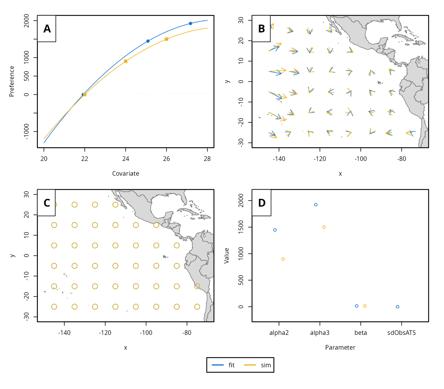
momo provides several functions for visualizing model results. In this example, since the data are simulated and the true parameters are known, we can use the plotmomo.compare function to visualize both the estimated and true habitat preferences and movement patterns.

Advanced settings

There are several advanced settings in momo that will be covered in future vignettes. However, this vignette highlights three important ones: (i) grouping tags into release events to speed up model fitting, (ii) using the matrix exponential approach as an alternative to the Kalman filter, and (iii) mapping parameters to fix or exclude them during estimation.

It is common for multiple tags to be released at the same location and time. Grouping these tags into release events can significantly speed up the movement modeling, as the analysis is performed per event rather than per individual tag. The potential loss in accuracy is likely minimal and can be evaluated through sensitivity analyses, while the grouped approach is recommended for the baseline scenario due to its efficiency. The get.release.event function enables this grouping by assigning tags to release events based on a specified spatial grid and time vector. These events can then be added to the data list for modeling. Note that this is step is optional.

By default, momo uses the Kalman filter approach as described in Mildenberger, Maunder, and Nielsen (in prep). However, it also supports an alternative method based on the matrix exponential. You can easily switch between the two by setting the use.expm flag in the configuration list. To use the matrix exponential approach, simply set use.expm = TRUE.

Lastly, it may be useful to map parameters, for example, to estimate a single value for both directions of passive advection. A list of default mapping settings can be generated using the def.map function. The resulting map can then be passed to fit.momo to control which parameters are estimated, fixed, or shared.

Summary

This vignette introduced the main features and workflow of the momo package for estimating animal movement and habitat preferences from tagging data. Using a simulated data set (skjepo), we demonstrated how to prepare the required inputs, configure and fit the model, and visualize the results.

We covered the preparation of conventional and archival tag data (prep.ctags, prep.atags), environmental fields (prep.env), and spatial grids (create.grid). These were then combined using setup.momo.data into a format suitable for model fitting. Configuration and parameter initialization were handled through def.conf and def.par, with model fitting performed using fit.momo. The plotmomo.compare function allowed us to visualize and compare estimated versus true movement and habitat preference patterns.

Several advanced options were introduced, including grouping tags into release events (get.release.event), switching between the Kalman filter and matrix exponential approaches (use.expm flag), and mapping parameters (def.map) to simplify or constrain estimation.

This basic example provides a foundation for applying momo to real tagging data. More details about the methodology are described in Mildenberger, Maunder, and Nielsen (in prep). Further details about functions and their arguments can be found in the help files of the functions (help() or ?, where the dots refer to any function of the package). Additional vignettes will explore uncertainty estimation, model diagnostics, and sensitivity analyses to support more robust ecological inference and management applications.

References

Mildenberger, Tobias Karl, Mark Maunder, and Anders Nielsen. in prep. “Momo: An r Package for the Estimation of Fine-Scale Animal Movement Based on Tagging Data.” Methods in Ecology and Evolution, in prep.