Data processing and quality control

library(DATRASextra)

Every DATRAS analysis rests on a chain of processing decisions: which hauls count as valid, how sub-sampled catches are raised, what a missing value looks like, and which records are dropped along the way. Most of those decisions are made before a user writes a single line of analysis code.

This vignette documents that chain end to end. For each step it states what is done, whether it happens automatically or on request, how to inspect its effect, and how to change or switch it off. It also lists checks that DATRASextra deliberately leaves to the user, because the right answer depends on the analysis.

Two principles guide the design:

Nothing is silently discarded. The mandatory filters in clean_datras() are the DATRAS-recommended minimum, and the function prints what will be removed before removing it.
Checks report, they do not delete. check_outliers(), check_lengths() and check_weights() are opt-in, and check_outliers() returns the object unchanged unless explicitly asked to remove hauls.

Overview of the pipeline

Stage	Function	What happens	Automatic?
1. Download	`download_datras()` (via `DATRAS::getDatrasExchange()`)	Query ICES web service, harmonise column names, convert the `-9` sentinel to `NA`, match orphan `CA` records, archive as exchange zip	automatic
2. Read	`read_datras()` (via `DATRAS::readICES()`)	Parse exchange CSV, drop truncated files, match orphan `CA` records, drop duplicated hauls, combine survey-years	automatic
3. Derived variables	`DATRAS::addExtraVariables()`	Create `haul.id`, `LngtCm`, `Species`, `Count`, `lon`/`lat`, `abstime`, `Roundfish`; treat hauls without `HL` records as zero-catch	automatic
4. Cleaning	`clean_datras()`	Filter on `HaulVal` and `StdSpecRecCode`, optionally impute depth and harmonise species, optionally subset	automatic filters, optional extras
5. Checks	`check_outliers()`, `check_lengths()`, `check_weights()`, `add_swept_area()`	Flag implausible values, summarise length and weight distributions, report swept-area missingness	opt-in
6. Inspection	`print()`, `summary()`, `plot_datras_overview()`, `plot_length_distribution()`, `plot_species_composition()`	Tabular and visual review	opt-in
7. Extraction record	`extraction()`, `write_manifest()`, `verify_extraction()`	Record where the data came from and detect upstream revisions	automatic record, opt-in verification

Throughout we use the bundled example data set mini: four surveys, nine gears, five species, 2015-2020. Unlike the dab example, mini has not been pre-cleaned, so every filter described below actually does something.

mini
#> Object of class 'datras_raw'
#> ===========================
#> Number of hauls: 13074 
#> Number of species: 5 
#> Number of surveys: 4 [BITS, BTS, EVHOE, NS-IBTS]
#> Number of gears: 9 
#> Number of countries: 14 
#> Years: 2015 - 2020 
#> Quarters: 1 2 3 4 
#> Longitude range: -11.28 - 22.2 deg
#> Latitude range: 43.69 - 61.78 deg
#> Depth range: 5 - 518 m
#> Haul duration: 0 - 1470 minutes
#> Valid hauls: 12520 (554 invalid)
#> Hauls with catch: 6134 (zero catch: 6940)
#> Extraction: 43 source(s), extracted 2026-10-09, ICES calculation 2016-04-16 to 2024-08-15

Stage 1: Download

download_datras() wraps DATRAS::getDatrasExchange(), which in turn queries the ICES DATRAS web service. Several things happen before anything reaches disk.

## One survey, selected years, archived under <path>/NS-IBTS/
x <- download_datras(path = "data/datras", surveys = "NS-IBTS", years = 2020:2023)

Which surveys and years are requested

Available surveys, years and quarters are read from the ICES web service. If the server does not answer within timeout seconds (default 10), the function falls back to a cached survey list and, for years, to whatever zip files are already present locally. This keeps a partially completed download resumable when the connection is unreliable, but it also means that an offline session may silently work from a stale survey list.

Two surveys are skipped by default because they are test entries or do not contain the full set of required tables: Test-DATRAS and NS-IBTS_UNIFtest. Set include_flagged = TRUE to download them anyway.

The download_hl and download_ca arguments control whether the length-frequency and biological tables are fetched at all. Omitting whichever table an analysis does not need reduces both download time and memory use; CA is the usual candidate, since many analyses need only catch-at-length.

Harmonisation applied on download

DATRAS::getDatrasExchange() applies the following, in order:

Column renaming (DATRAS::renameDATRAS()). Names are capitalised, and the web-service names are mapped onto the exchange-format names: ValidAphiaID becomes Valid_Aphia, LngtClass becomes LngtClas, AgeRings becomes Age, and CANoAtLngt / NoAtLngt become NoAtALK. This is why the same variable has different names in the ICES documentation and in an R object.
Missing-value conversion (DATRAS::minus9toNA()). DATRAS encodes missing numeric values as -9. Every numeric column is scanned and -9 is replaced by NA. Note that this applies to numeric columns only: a -9 stored as text is left untouched.
StatRec back-fill. If the CA table has no StatRec column, it is filled from AreaCode.
Derived variables are added (see Stage 3 below).
Orphan CA records are matched back to hauls with DATRAS::fixMissingHaulIds() using strict = TRUE, so ambiguous records are left unmatched rather than attributed to an arbitrary haul.
Character columns are converted to factors.

What gets archived

Before writing, download_datras() strips the derived columns again and maps the names back to the exchange-format spelling, so the archived zip is a faithful DATRAS exchange file rather than an R-specific artefact. Anyone can re-read it, with DATRASextra or with any other tool that understands the exchange format. Files are named <survey>_<year>.zip inside a per-survey subdirectory.

This separation matters for reproducibility: the archive is the raw record, and every processing step described in the rest of this vignette is reapplied from it each time the data are read. Alongside the zip files, download_datras() maintains DATRAS_manifest.csv, recording the extraction date, a checksum and the ICES calculation date of every survey-year-quarter it retrieved; see Recording and verifying the extraction below.

## Re-download and replace existing files
download_datras(path = "data/datras", surveys = "NS-IBTS", years = 2020,
                overwrite = TRUE)

Worth checking after a download: that a file exists for every year you expect, and that none of them is suspiciously small. read_datras() performs the size check for you (next section), but an unexpectedly missing year usually means the survey was not conducted rather than that the download failed.

Stage 2: Reading data into R

x <- read_datras("data/datras", surveys = "NS-IBTS", years = 2020:2023)

Parsing and file-level checks

A DATRAS exchange CSV contains three stacked blocks, each with its own header line. DATRAS::readICES() locates the header lines, reads each block separately, and applies na.strings = c("-9", "-9.0", "-9.00", "-9.0000") so that the missing-value sentinel is converted on the way in. It then verifies that the number of data rows plus header lines equals the number of lines in the file, and aborts with "csv file appears to be corrupt" if it does not.

read_datras() reads each file separately. A file that cannot be read, for example a truncated download, is skipped with a message giving the reason, and the remaining files are still read. Exact duplicates of an HH record, which make DATRAS::readICES() reject the whole file, are removed and reported first. Empty files are skipped; min_file_size (default 0 bytes) raises that threshold. download_datras() writes no file for a year without hauls.

Matching biological records to hauls: the `strict` argument

Records in CA frequently lack the station and haul numbers that make up haul.id. DATRAS::fixMissingHaulIds() matches them back to a haul using survey, year, quarter, country, ship and statistical rectangle. When that combination identifies more than one candidate haul, the two settings diverge:

strict = FALSE assigns the record to one of the candidate hauls at random.
strict = TRUE leaves the record as NA, and it is dropped by any subsequent subsetting.

Which behaviour is right depends on the analysis: random assignment preserves sample size for aggregate age-length keys, while leaving records unmatched is the honest choice when individual records must be attributable to a specific haul.

## Attribute ambiguous CA records to an arbitrary haul
x <- read_datras("data/datras", strict = FALSE)

Combining survey-year files

Files are read one at a time and combined. Two safeguards apply:

Duplicated haul identifiers. The same haul appearing in more than one file is reported by haul.id and removed. Note that the two code paths behave slightly differently: the sequential reader (ncores = 1) keeps the first copy encountered and drops later ones, while the parallel reader removes all copies. If duplicates are reported, the underlying archive is worth investigating rather than accepting either behaviour.
Type-consistent binding. c.datras_raw() guards against a column that is a factor in one year and an integer in another. Plain rbind() would use the factor’s level vector as the type and reinterpret the other year’s integers as factor codes, silently turning valid values into NA.

For large reads, prune = TRUE, drop_hl = TRUE and drop_ca = TRUE reduce peak memory by trimming columns or dropping whole tables inside the reader, and surveys / years restrict which files are opened at all.

Stage 3: Variables created while reading

The columns most analyses actually use are not in the exchange file at all: they are constructed by DATRAS::addExtraVariables() during both download and read.

Haul identifier

haul.id = Survey:Year:Quarter:Country:Ship:Gear:StNo:HaulNo

This is the key that links HH, HL and CA.

head(levels(mini[["HH"]]$haul.id), 3)
#> [1] "BITS:2015:1:DE:06SL:TVS:22002:1" "BITS:2015:1:DE:06SL:TVS:22004:7"
#> [3] "BITS:2015:1:DE:06SL:TVS:22005:4"

Length in centimetres

LngtClas is reported in units that depend on LngtCode. The conversion to LngtCm uses:

`LngtCode`	Multiplier for `LngtClas`	Meaning
`.`	0.1	reported in mm
`0`	0.1	reported in mm, 0.5 cm classes
`1`	1	reported in cm, 1 cm classes
`2`	1	reported in cm, 2 cm classes
`5`	1	reported in cm, 5 cm classes

There is a trap here worth stating explicitly. A second, different table with the same codes is used by get_accuracy_cm() (and DATRAS::getAccuracyCM()) to describe the bin width: . = 0.1, 0 = 0.5, 1 = 1, 2 = 2, 5 = 5. The first table converts a recorded value to centimetres; the second says how wide the length class is. They are not interchangeable.

## Which length codes occur, and what resolution do they imply
table(mini[["HL"]]$LngtCode, useNA = "ifany")
#> 
#>     .     0     1  <NA> 
#> 39656   557 44270    62

## The coarsest resolution present is used for automatic length binning
get_accuracy_cm(mini)
#> Warning in get_accuracy_cm(mini): Mixed accuracies found in var[[3]]$LngtCode -
#> worst chosen: 1 cm
#> Warning in get_accuracy_cm(mini): NAs found in var[[3]]$LngtCode - assumed to
#> be 1 cm
#> [1] 1

Mixed codes are common when several surveys or countries are combined, and get_accuracy_cm() warns and falls back to the coarsest resolution. Empty LngtCode values are assumed to be 1 cm. If that assumption is wrong for your data, pass cm_breaks or by explicitly to the length functions rather than relying on the automatic choice.

Species names

Species is resolved from SpecCode using either an ITIS/TSN lookup table or a WoRMS lookup table, depending on whether SpecCodeType is "W". Older survey years often use TSN codes while recent years use WoRMS codes, so both paths can occur in a single combined object.

table(mini[["HL"]]$SpecCodeType, useNA = "ifany")
#> 
#>     W 
#> 84545

Raised catch numbers

This is the most consequential derived variable:

Count = HLNoAtLngt * (HaulDur / 60 if DataType == "C", else 1) * SubFactor

Two corrections are folded into one column:

Sub-sampling. SubFactor raises the measured sub-sample to the whole catch.
Standardisation of reporting units. DataType == "C" means numbers were reported per hour, so they are converted back to per-haul using the haul duration. DataType == "R" (raw) and "P" are used as reported.

A combined object frequently mixes reporting conventions:

table(mini[["HH"]]$DataType, useNA = "ifany")
#> 
#>    C    R    P <NA> 
#> 3587 9177  303    7

Anything computed from Count therefore already accounts for sub-sampling and per-hour reporting. Recomputing from HLNoAtLngt without applying both corrections is a common source of error. Note also that check_lengths() warns if DataType == "S" is present, since those hauls are treated as "R".

Time and position

lon and lat are copies of ShootLong and ShootLat, that is the position where the gear was shot, not the midpoint of the tow. HaulLat and HaulLong hold the end position if a tow midpoint is needed.
abstime is a decimal year, timeOfYear its fractional part, and TimeShotHour the time of day in decimal hours. These are convenient for smoothers over time or time of day.
Roundfish is the North Sea roundfish area, derived from StatRec.

Hauls without catch records

Any haul present in HH that has no rows in HL is interpreted as a zero-catch haul. During reading, the upstream code prints a warning listing the affected hauls. This is the correct treatment for a species-restricted extract such as mini, where most hauls simply did not catch the five target species, but it means a haul missing from HL for a data-handling reason is indistinguishable from a genuine zero.

The split is reported by print():

mini
#> Object of class 'datras_raw'
#> ===========================
#> Number of hauls: 13074 
#> Number of species: 5 
#> Number of surveys: 4 [BITS, BTS, EVHOE, NS-IBTS]
#> Number of gears: 9 
#> Number of countries: 14 
#> Years: 2015 - 2020 
#> Quarters: 1 2 3 4 
#> Longitude range: -11.28 - 22.2 deg
#> Latitude range: 43.69 - 61.78 deg
#> Depth range: 5 - 518 m
#> Haul duration: 0 - 1470 minutes
#> Valid hauls: 12520 (554 invalid)
#> Hauls with catch: 6134 (zero catch: 6940)
#> Extraction: 43 source(s), extracted 2026-10-09, ICES calculation 2016-04-16 to 2024-08-15

The ICES calculation date

One column is neither derived nor really part of the survey data: DateofCalculation, the date on which ICES last recalculated the records. It is constant per survey, year and quarter, and it is the only field that reveals that the database has been revised since a download. It is discussed in Recording and verifying the extraction below.

with(mini[["HH"]], table(Survey, DateofCalculation))
#>          DateofCalculation
#> Survey    20160416 20170316 20170914 20180423 20180507 20190305 20190307
#>   BITS           0        0        0        0        0        0        0
#>   BTS            0        0        0        0        0        0        0
#>   EVHOE        150        0        0       26      161      155        0
#>   NS-IBTS        0      369      374        0        0        0       10
#>          DateofCalculation
#> Survey    20200219 20200408 20200525 20210222 20210304 20210428 20210607
#>   BITS           0      296        0        0        0      333        0
#>   BTS            0        0     1339        0      162        0        0
#>   EVHOE        151        0        0      156        0        0        0
#>   NS-IBTS        0        0        0        0        0        0      387
#>          DateofCalculation
#> Survey    20211004 20211029 20211209 20220125 20220407 20220408 20220411
#>   BITS           0        0        0        0      318        0        0
#>   BTS            0        0     1301        0        0        0     1400
#>   EVHOE          0        0        0        0        0        0        0
#>   NS-IBTS      362      349        0     1070        0      362        0
#>          DateofCalculation
#> Survey    20220422 20220427 20220712 20230322 20240712 20240809 20240814
#>   BITS         242      297        0        0      311      302      625
#>   BTS            0        0        0        0        0        0        0
#>   EVHOE          0        0        0        0        0        0        0
#>   NS-IBTS        0        0      372      775        0        0        0
#>          DateofCalculation
#> Survey    20240815
#>   BITS         919
#>   BTS            0
#>   EVHOE          0
#>   NS-IBTS        0

Type coercions to be aware of

Year and Quarter are converted to factors. mini[["HH"]]$Year + 1 does not do what it looks like; use as.integer(as.character(Year)).
All character columns become factors.
haul.id in HL and CA is re-levelled to the levels present in HH, so records that do not correspond to a haul in HH become NA and are dropped by later subsetting.
Duplicated rows in HH abort the read entirely with "Duplicated rows found in HH data - data file is corrupt".

Stage 4: Cleaning with `clean_datras()`

clean_datras() applies the standard DATRAS cleaning filters. With verbose = TRUE (the default) it prints a full account of the data before filtering, and explain_codes = TRUE adds the meaning of each code.

surv <- clean_datras(mini, explain_codes = TRUE)
#> HaulVal (13074 hauls before cleaning):
#> Code      n  Description                                              
#>    A     60  Additional valid stations not used for index calculations
#>    I    275  Invalid haul                                             
#>    N    219  No oxygen (BITS only)                                    
#>    V  12520  Valid haul
#> 
#> StdSpecRecCode:
#> Code      n  Description                         
#>    0     39  No standard species recorded        
#>    1  13015  All standard species recorded       
#>    3     10  Roundfish standard species recorded 
#>    4     10  Individual standard species recorded
#> 
#> BySpecRecCode:
#> Code      n  Description                 
#>    0    170  No bycatch species recorded 
#>    1  12904  All bycatch species recorded
#> 
#> Hauls with missing lon: 0
#> Hauls with missing lat: 0
#> Hauls with missing Year: 0
#> Hauls with missing Depth: 67
#> Hauls with missing HaulDur: 0
#> Hauls with missing Distance: 739
#> Hauls with missing GroundSpeed: 2501
#> Hauls with missing WingSpread: 8889
#> Hauls with missing DoorSpread: 5515
#> 
#> Hauls removed by HaulVal filter: 335
#> Hauls removed by StdSpecRecCode filter: 14
#> Hauls remaining: 12725
#> 
#> Note: 219 retained haul(s) have HaulVal = "N" (no oxygen, BITS only) and may have unusually short HaulDur.

The report has three parts: the distribution of the three recording codes, the missing-value counts for the variables that later steps depend on, and the number of hauls removed by each filter.

Filter 1: haul validity

Only hauls with HaulVal in c("V", "N") are retained.

Code	Meaning	Kept
`V`	Valid haul	yes
`N`	No oxygen (BITS only)	yes
`S`	Standard haul	no
`A`	Additional valid station, not used for index calculations	no
`C`	Calibrated (BITS only)	no
`I`	Invalid haul	no
`M`	Pelagic midwater trawl (BITS only)	no
`P`	Partly valid haul (sensor problems)	no

"N" hauls are Baltic stations aborted because of oxygen depletion. They are retained because the catch is valid for the duration fished, but they often have an unusually short HaulDur, and clean_datras() says so when any are kept. Whether to keep them is an analysis decision: they are legitimate observations, but a swept-area index that does not account for the shorter tow will be biased.

Filter 2: standard species recording

Only records with StdSpecRecCode == 1 (“all standard species recorded”) are retained. Codes 2, 3 and 4 mean that only pelagic, roundfish or individual standard species were recorded, and 0 means none were. Keeping them would mix hauls with different species coverage, which biases community-level and multi-species analyses.

Note what is not filtered. BySpecRecCode is reported but never used as a filter: bycatch recording protocols differ by survey, and which species are usable under each code is an analysis-specific judgement. The relevant per-code species lists exist in the source of correct_species() as reference material but are deliberately inactive.

Optional: imputing missing depths

Disabled by default. When enabled, missing Depth values are predicted from a GAM of log(Depth) on a two-dimensional smooth of longitude and latitude, using the hauls that do have a recorded depth. This requires the R package mgcv.

surv_dep <- clean_datras(mini, impute_missing_depth = TRUE, verbose = FALSE)

## Missing depths before and after
c(before = sum(is.na(mini[["HH"]]$Depth)),
  after = sum(is.na(surv_dep[["HH"]]$Depth)))
#> before  after 
#>     67      0

The imputed values replace NA in place, and there is no flag distinguishing them afterwards. If that distinction matters, record the affected haul identifiers before cleaning:

imputed_ids <- as.character(mini[["HH"]]$haul.id[is.na(mini[["HH"]]$Depth)])
imputed_ids
#>  [1] "BTS:2015:3:DE:06SL:BT7:640:6"       "BTS:2018:3:NL:64T2:BT8:33F428:128" 
#>  [3] "BTS:2019:3:DE:06SL:BT7:655:1"       "BTS:2019:3:DE:06SL:BT7:656:2"      
#>  [5] "BTS:2019:3:DE:06SL:BT7:657:3"       "BTS:2019:3:DE:06SL:BT7:658:4"      
#>  [7] "BTS:2019:3:DE:06SL:BT7:659:5"       "BTS:2019:3:DE:06SL:BT7:660:6"      
#>  [9] "BTS:2019:3:DE:06SL:BT7:671:17"      "BTS:2019:3:DE:06SL:BT7:672:18"     
#> [11] "BTS:2019:3:DE:06SL:BT7:673:19"      "BTS:2019:3:DE:06SL:BT7:674:20"     
#> [13] "BTS:2019:3:DE:06SL:BT7:675:21"      "BTS:2019:3:DE:06SL:BT7:676:22"     
#> [15] "BTS:2019:3:DE:06SL:BT7:677:23"      "BTS:2019:3:DE:06SL:BT7:678:24"     
#> [17] "BTS:2019:3:DE:06SL:BT7:679:25"      "BTS:2019:3:DE:06SL:BT7:680:26"     
#> [19] "BTS:2019:3:DE:06SL:BT7:681:27"      "BTS:2019:3:DE:06SL:BT7:682:28"     
#> [21] "BTS:2019:3:DE:06SL:BT7:683:29"      "BTS:2019:3:DE:06SL:BT7:684:30"     
#> [23] "BTS:2019:3:DE:06SL:BT7:685:31"      "BTS:2019:3:DE:06SL:BT7:686:32"     
#> [25] "BTS:2019:3:DE:06SL:BT7:687:33"      "BTS:2019:3:DE:06SL:BT7:688:34"     
#> [27] "BTS:2019:3:DE:06SL:BT7:689:35"      "BTS:2019:3:DE:06SL:BT7:690:36"     
#> [29] "BTS:2019:3:DE:06SL:BT7:691:37"      "BTS:2019:3:DE:06SL:BT7:692:38"     
#> [31] "BTS:2019:3:DE:06SL:BT7:693:39"      "BTS:2019:3:DE:06SL:BT7:694:40"     
#> [33] "BTS:2019:3:DE:06SL:BT7:695:41"      "BTS:2019:3:DE:06SL:BT7:696:42"     
#> [35] "BTS:2019:3:DE:06SL:BT7:697:43"      "BTS:2019:3:DE:06SL:BT7:698:44"     
#> [37] "BTS:2019:3:DE:06SL:BT7:699:45"      "BTS:2019:3:DE:06SL:BT7:700:46"     
#> [39] "BTS:2019:3:DE:06SL:BT7:701:47"      "BTS:2019:3:DE:06SL:BT7:702:48"     
#> [41] "BTS:2019:3:DE:06SL:BT7:703:49"      "BTS:2019:3:DE:06SL:BT7:704:50"     
#> [43] "BTS:2019:3:DE:06SL:BT7:705:51"      "BTS:2019:3:DE:06SL:BT7:706:52"     
#> [45] "BTS:2019:3:DE:06SL:BT7:707:53"      "BTS:2019:3:DE:06SL:BT7:708:54"     
#> [47] "BTS:2019:3:DE:06SL:BT7:709:55"      "BTS:2019:3:DE:06SL:BT7:710:56"     
#> [49] "BTS:2019:3:DE:06SL:BT7:711:57"      "BTS:2019:3:DE:06SL:BT7:712:58"     
#> [51] "BTS:2019:3:DE:06SL:BT7:713:59"      "BTS:2019:3:DE:06SL:BT7:714:60"     
#> [53] "BTS:2019:3:DE:06SL:BT7:715:61"      "BTS:2019:3:DE:06SL:BT7:716:62"     
#> [55] "BTS:2019:3:DE:06SL:BT7:717:63"      "BTS:2019:3:DE:06SL:BT7:718:64"     
#> [57] "BTS:2019:3:DE:06SL:BT7:719:65"      "BTS:2019:3:DE:06SL:BT7:720:66"     
#> [59] "BTS:2019:3:DE:06SL:BT7:721:67"      "BTS:2019:3:DE:06SL:BT7:722:68"     
#> [61] "BTS:2019:3:DE:06SL:BT7:723:69"      "BTS:2019:3:DE:06SL:BT7:724:70"     
#> [63] "BTS:2019:3:DE:06SL:BT7:725:71"      "BTS:2019:3:DE:06SL:BT7:726:72"     
#> [65] "BTS:2019:3:DE:06SL:BT7:727:73"      "EVHOE:2019:4:FR:35HT:GOV:X0441:1"  
#> [67] "EVHOE:2019:4:FR:35HT:GOV:X0550:104"

Spatial interpolation of depth is reasonable on a continental shelf and poor across a shelf break. Inspect the result before relying on it.

Optional: harmonising species

correct_species = TRUE (the default) calls correct_species(), which does two things.

First, it collapses taxa that are not reliably identified to species in the field down to genus level, updating Species, Valid_Aphia and Rank: Dipturus, Liparis, Chelon, Mustelus, Alosa, Argentina, Callionymus, Ciliata, Gaidropsarus, Sebastes, Syngnatus, Pomatoschistus and Gobius. Records identified as Nerophis ophidion, Leusueurigobius, Neogobius and Argentinidae are folded into the corresponding genus.

Second, it corrects outdated or misspelled names: Synaphobranchus kaupi becomes Synaphobranchus kaupii, and Dipturus linteus becomes Rajella lintea with the current AphiaID.

The Rank column it adds makes the outcome visible:

table(surv[["HL"]]$Rank, useNA = "ifany")
#> 
#> species 
#>   84169

Set correct_species = FALSE to keep the original species assignments, for example when reproducing an earlier analysis or when comparing against the raw ICES extract.

Optional: subsetting

aphias, years, quarters and gears are applied after the filters, as a convenience:

surv_sub <- clean_datras(mini, years = 2020, quarters = 1,
                         aphias = 127137, verbose = FALSE)
surv_sub
#> Object of class 'datras_raw'
#> ===========================
#> Number of hauls: 811 
#> Number of species: 1 [Hippoglossoides platessoides (127137)]
#> Number of surveys: 3 [BITS, BTS, NS-IBTS]
#> Number of gears: 5 
#> Number of countries: 11 
#> Years: 2020 - 2020 
#> Quarters: 1 
#> Longitude range: -6.62 - 21.34 deg
#> Latitude range: 48.69 - 61.74 deg
#> Depth range: 10 - 256 m
#> Haul duration: 0 - 40 minutes
#> Valid hauls: 787 (24 invalid)
#> Hauls with catch: 254 (zero catch: 557)
#> Extraction: 3 source(s), extracted 2026-10-09, ICES calculation 2021-03-04 to 2022-04-07

Modifying or omitting steps

Step	Argument	Default	Effect of changing
Pre-cleaning report	`verbose`	`TRUE`	`FALSE` silences it, for scripts
Code descriptions	`explain_codes`	`FALSE`	`TRUE` annotates each code
Haul validity filter	none	always applied	reproduce manually with `subset()`
Standard species filter	none	always applied	reproduce manually with `subset()`
Depth imputation	`impute_missing_depth`	`FALSE`	`TRUE` fills missing depths by GAM
Species harmonisation	`correct_species`	`TRUE`	`FALSE` leaves names untouched
Subsetting	`aphias`, `years`, `quarters`, `gears`	`NULL`	applied after filtering
Alternative pipeline	`do_fishglob`	`FALSE`	`TRUE` delegates to `clean_fishglob()`

The two mandatory filters have no on/off switch, but they are ordinary subset() calls and are trivially replaced when a different rule is wanted:

## Keep additional valid stations as well as valid and no-oxygen hauls
custom <- subset(mini, HaulVal %in% c("V", "N", "A"))

## Accept hauls where only individual standard species were recorded
custom <- subset(custom, StdSpecRecCode %in% c(1, 4))

## Then apply the optional steps only
custom <- correct_species(custom)
custom
#> Object of class 'datras_raw'
#> ===========================
#> Number of hauls: 12789 
#> Number of species: 5 
#> Number of surveys: 4 [BITS, BTS, EVHOE, NS-IBTS]
#> Number of gears: 9 
#> Number of countries: 14 
#> Years: 2015 - 2020 
#> Quarters: 1 2 3 4 
#> Longitude range: -11.28 - 22.2 deg
#> Latitude range: 43.69 - 61.75 deg
#> Depth range: 5 - 518 m
#> Haul duration: 0 - 1470 minutes
#> Valid hauls: 12515 (274 invalid)
#> Hauls with catch: 6114 (zero catch: 6675)
#> Extraction: 43 source(s), extracted 2026-10-09, ICES calculation 2016-04-16 to 2024-08-15

Compare the haul count with surv above to see what the relaxed rule buys, and decide whether the extra stations are usable for your purpose.

For the FishGlob workflow, do_fishglob = TRUE replaces the whole cleaning stage with clean_fishglob(); see vignette("articles/fishglob").

Stage 5: Quality-control checks

These functions are deliberately not called by clean_datras(). They flag values that are implausible rather than formally invalid, and whether a flagged record should be excluded is a decision the analyst has to make.

`check_outliers()`

Two independent mechanisms, both optional to act on.

Rule-based checks

Fixed, physically motivated bounds. strict = TRUE is the default; FALSE relaxes the upper bounds.

Table	Variable	Rule (`strict = TRUE`)	Rule (`strict = FALSE`)
`HH`	`Quarter`	outside 1-4	same
`HH`	`Year`	before 1965 or in the future	same
`HH`	`TimeShot`	not a valid HHMM time	same
`HH`	`HaulDur`	outside 0-240 min	outside 0-360 min
`HH`	`ShootLat`	outside -90 to 90	same
`HH`	`ShootLong`	outside -180 to 180	same
`HH`	`Depth`	outside 0-2000 m	outside 0-3000 m
`HH`	`GroundSpeed`	outside 0-6 knots	outside 0-8 knots
`HH`	`DoorSpread`	outside 0-250 m	outside 0-300 m
`HH`	`WingSpread`	outside 0-80 m	outside 0-120 m
`HH`	`WingSpread`, `DoorSpread`	wing spread exceeds door spread	same
`HL`	`LngtCm`	outside 0-200 cm	outside 0-300 cm
`CA`	`Sex`	not in `""`, `F`, `M`, `U`	same
`CA`	`Age`	outside 0-50, or non-integer	outside 0-80
`CA`	`NoAtALK`	negative or non-integer	same
`CA`	`IndWgt`	outside 0-1e5 g	outside 0-3e5 g
`CA`	`LngtCode`	not in `""`, `.`, `0`, `1`	same
`CA`	`LngtClas`	outside 0-2000, or non-integer	outside 0-3000

Rule violations get severity "invalid".

Percentile checks

Enabled with pct = TRUE. Within groups, values outside the requested percentiles are flagged with severity "extreme". Defaults:

pct_probs = c(0.01, 0.99)
pct_by: HH grouped by survey, quarter, gear and ship; HL and CA by survey, quarter, gear and species
pct_vars: HaulDur, Depth, DoorSpread, WingSpread in HH; LngtCm in HL; Age, IndWgt, LngtClas in CA
pct_min_n = 50: groups with fewer observations are skipped rather than producing unstable thresholds
pct_log_vars: IndWgt percentiles are computed on the log scale

Grouping matters. Comparing a beam trawl against a GOV trawl on the same threshold produces nonsense; the defaults compare like with like.

Running the checks

surv <- check_outliers(surv, pct = TRUE)
#> Detected 3312 flagged row(s) in 1627 haul(s). (includes percentile checks)
#>    table                   var severity  one
#> 1     CA                   Age  extreme  115
#> 2     HH                 Depth  extreme  246
#> 3     HH            DoorSpread  extreme  139
#> 4     HH               HaulDur  extreme  117
#> 5     CA                IndWgt  extreme  454
#> 6     CA              LngtClas  extreme 1033
#> 7     HL                LngtCm  extreme 1052
#> 8     HH            WingSpread  extreme   70
#> 9     HH            DoorSpread  invalid    7
#> 10    HH           GroundSpeed  invalid   17
#> 11    HH               HaulDur  invalid   54
#> 12    HH            WingSpread  invalid    2
#> 13    HH WingSpread,DoorSpread  invalid    6

By default nothing is removed: the object comes back unchanged, with four attributes attached.

## Every flagged record, one row each
report <- attr(surv, "outlier_report")
dim(report)
#> [1] 3312   13
head(report[report$severity == "invalid", c("table", "var", "value", "reason")])
#>   table     var value                    reason
#> 1    HH HaulDur     0 HaulDur outside 0-240 min
#> 2    HH HaulDur     0 HaulDur outside 0-240 min
#> 3    HH HaulDur     0 HaulDur outside 0-240 min
#> 4    HH HaulDur     0 HaulDur outside 0-240 min
#> 5    HH HaulDur     0 HaulDur outside 0-240 min
#> 6    HH HaulDur     0 HaulDur outside 0-240 min

The report columns are: table, var, row, haul.id, value, reason, method ("rule" or "percentile"), severity ("invalid" or "extreme"), p_lo / p_hi (the percentiles used), thr_lo / thr_hi (the resulting thresholds) and group (the grouping key).

Three further attributes hold the affected haul identifiers:

c(all = length(attr(surv, "outlier_hauls")),
  invalid = length(attr(surv, "outlier_hauls_invalid")),
  extreme = length(attr(surv, "outlier_hauls_extreme")))
#>     all invalid extreme 
#>    1627      79    1567

Which variables drive the flags:

with(report, table(var, severity))
#>                        severity
#> var                     extreme invalid
#>   Age                       115       0
#>   Depth                     246       0
#>   DoorSpread                139       7
#>   GroundSpeed                 0      17
#>   HaulDur                   117      54
#>   IndWgt                    454       0
#>   LngtClas                 1033       0
#>   LngtCm                   1052       0
#>   WingSpread                 70       2
#>   WingSpread,DoorSpread       0       6

Acting on the results

## Remove only the rule-based failures; percentile flags are kept
cleaned <- check_outliers(surv, action = "remove", verbose = FALSE)
nrow(cleaned[["HH"]])
#> [1] 12646

remove_extremes = TRUE additionally removes the percentile-flagged hauls, but that is rarely appropriate: with pct_probs = c(0.01, 0.99), roughly two per cent of the data is flagged by construction, whether or not anything is wrong. The flags are a place to start looking, not a verdict.

Narrower or stricter runs:

## Only check the variables that feed the swept-area calculation
sa_check <- check_outliers(surv, vars = c("HaulDur", "Distance", "GroundSpeed",
                                          "DoorSpread", "WingSpread"),
                           pct = TRUE, pct_probs = c(0.005, 0.995),
                           verbose = FALSE)
nrow(attr(sa_check, "outlier_report"))
#> [1] 260

A threshold of your own is usually easier to apply to the report than to express as a new rule. The report gives you the haul identifiers, so any selection can be turned into a subset:

## Hauls flagged for haul duration, by method
subset(report, var == "HaulDur")[c("value", "method", "thr_lo", "thr_hi")][1:5, ]
#>   value method thr_lo thr_hi
#> 1     0   rule     NA     NA
#> 2     0   rule     NA     NA
#> 3     0   rule     NA     NA
#> 4     0   rule     NA     NA
#> 5     0   rule     NA     NA

## Your own threshold: hauls shorter than 15 minutes
short_ids <- unique(report$haul.id[report$var == "HaulDur" &
                                   as.numeric(report$value) < 15])
#> Warning in unique(report$haul.id[report$var == "HaulDur" &
#> as.numeric(report$value) < : NAs introduced by coercion
length(short_ids)
#> [1] 69

## Drop them if you decide they are unusable
nrow(subset(surv, !haul.id %in% short_ids)[["HH"]])
#> [1] 12656

`check_lengths()`

Summarises the pooled length distribution of a single species and compares the observed range with the empirical maximum length from the bundled species_info table.

plaice <- subset(surv, Valid_Aphia == 127137)
plaice <- check_lengths(plaice)
#> [1] "Length statistics:"
#>          min  mean median maxObs maxEmp perc
#> 99.9999%   1 15.62   15.5     50   82.6 50.5
#> [1] "Observations above:"
#>         maxLEmp percL
#> Numbers       0     0
#> Percent       0     0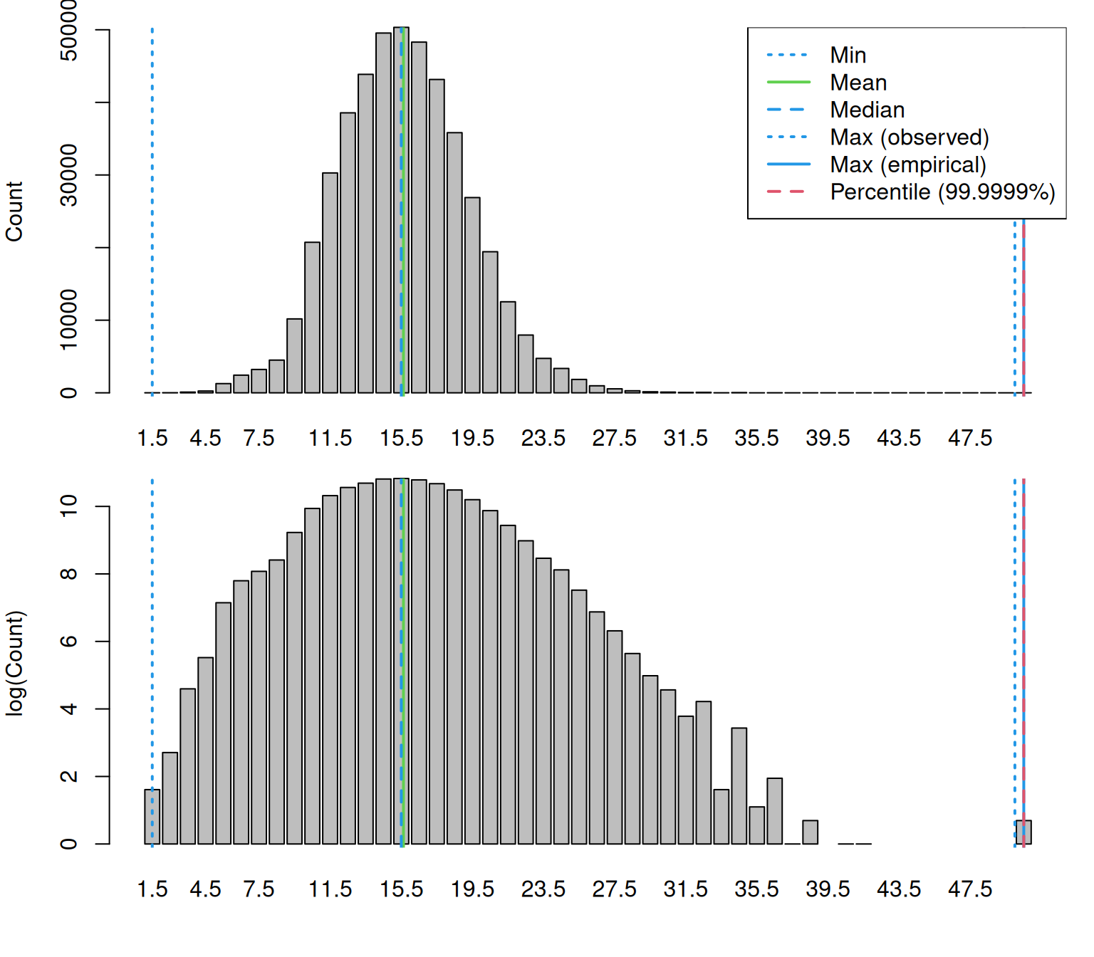

attr(plaice, "length_check")$lPars
#>          min     mean median maxObs maxEmp perc
#> 99.9999%   1 15.62306   15.5     50   82.6 50.5
attr(plaice, "length_check")$nAbove
#>         maxLEmp percL
#> Numbers       0     0
#> Percent       0     0

maxEmp is the published maximum length for the species (from FishBase); perc is the requested upper percentile of the observed distribution (length_percentile, default 99.9999). nAbove gives the number and percentage of observations above each. A non-trivial count above maxEmp points at length-unit errors or misidentification. Use cm_breaks or by to control the binning, and plot = FALSE to skip the figure.

`check_weights()`

Fits a log-log length-weight relationship to the individual weights in CA and compares it with the lookup parameters in species_info.

plaice <- add_numbers_at_length(plaice)
plaice <- check_weights(plaice)
#> [1] "Length statistics:"
#>   min  mean median  max
#> 1 8.4 18.22   18.2 31.6
#> [1] "Weight statistics:"
#>   min  mean median max
#> 1   4 52.16     42 245
#> [1] "Estimated LW parameters:"
#> [1] "a = 0.005 b = 3.122"
#> [1] "Lookup LW parameters in the species_info table:"
#> [1] "a = 0.004 b = 3.245"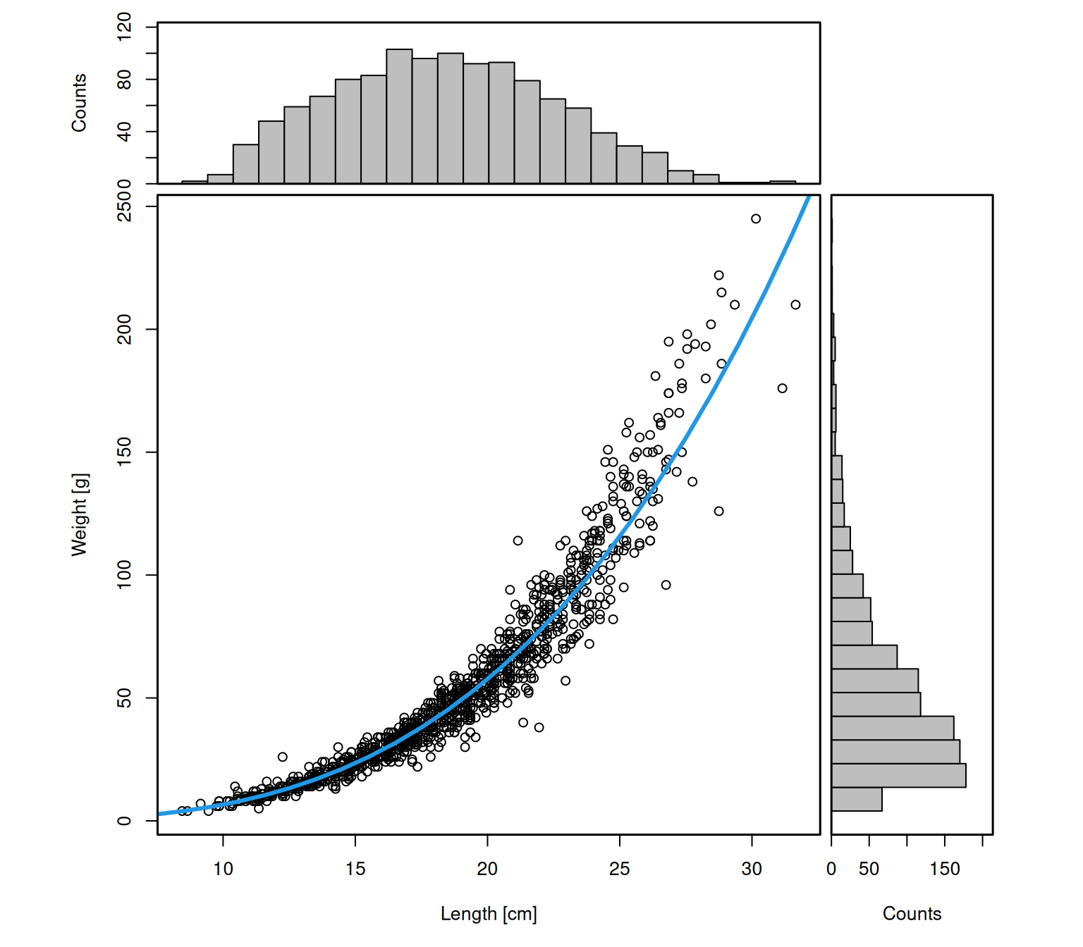

rbind(fitted = attr(plaice, "weight_check")$parEst,
      lookup = attr(plaice, "weight_check")$parEmp)
#>                  a        b
#> fitted 0.004996044 3.122263
#> lookup 0.003900000 3.244550

A fitted exponent b far from 3, or a large discrepancy against the lookup values, usually indicates unit errors or contaminated records. max_length and max_weight exclude implausible observations before fitting:

plaice2 <- check_weights(plaice, max_length = 60, max_weight = 5000)
#> [1] "Length statistics:"
#>   min  mean median  max
#> 1 8.4 18.22   18.2 31.6
#> [1] "Weight statistics:"
#>   min  mean median max
#> 1   4 52.16     42 245
#> [1] "Estimated LW parameters:"
#> [1] "a = 0.005 b = 3.122"
#> [1] "Lookup LW parameters in the species_info table:"
#> [1] "a = 0.004 b = 3.245"
attr(plaice2, "weight_check")$parEst
#>             a        b
#> 1 0.004996044 3.122263

`add_swept_area()`

Swept area is where survey data are at their most incomplete, so the function reports what it had to invent.

surv_sa <- add_swept_area(surv, full_report = TRUE)
#> Swept-area missingness and imputation by survey and gear:
#>   survey  gear n_records n_imputed prop_imputed n_NA prop_NA na_DoorSpread
#>     BITS   TVL      2105      1538        0.731    0   0.000           893
#>     BITS   TVS      1441      1419        0.985    0   0.000           199
#>      BTS  BT4A       693         0        0.000    0   0.000           693
#>      BTS BT4AI       561         0        0.000    0   0.000           561
#>      BTS  BT4P       729         0        0.000    0   0.000           729
#>      BTS  BT4S       836         0        0.000    0   0.000           836
#>      BTS   BT7       378         1        0.003    0   0.000           378
#>      BTS   BT8       895         0        0.000   12   0.013           895
#>    EVHOE   GOV       790        24        0.030    0   0.000            53
#>  NS-IBTS   GOV      4297      1612        0.375    0   0.000           101
#>  na_WingSpread na_Distance na_HaulDur na_GroundSpeed
#>           1535         475          0            298
#>           1419         210          0             76
#>            693           0          0            226
#>            561           0          0              0
#>            729           0          0              0
#>            836           0          0            108
#>            378           0          0              0
#>            895          12          0            895
#>             15           0          0            487
#>           1577          17          0            336

The summary is attached as an attribute and also gives a per-haul flag:

head(attr(surv_sa, "swept_area_summary"))
#>   survey  gear n_records n_imputed prop_imputed n_NA prop_NA na_DoorSpread
#> 1   BITS   TVL      2105      1538        0.731    0       0           893
#> 2   BITS   TVS      1441      1419        0.985    0       0           199
#> 3    BTS  BT4A       693         0        0.000    0       0           693
#> 4    BTS BT4AI       561         0        0.000    0       0           561
#> 5    BTS  BT4P       729         0        0.000    0       0           729
#> 6    BTS  BT4S       836         0        0.000    0       0           836
#>   na_WingSpread na_Distance na_HaulDur na_GroundSpeed
#> 1          1535         475          0            298
#> 2          1419         210          0             76
#> 3           693           0          0            226
#> 4           561           0          0              0
#> 5           729           0          0              0
#> 6           836           0          0            108

## Share of hauls whose spread or distance was imputed
mean(surv_sa[["HH"]]$SweptArea_imputed)
#> [1] 0.3610216

Read the table by survey and gear rather than in aggregate. A gear with prop_NA of 1 records neither of the required fields and cannot be given a swept area at all; a gear with a high prop_imputed has swept areas built from gear-level medians rather than haul-specific measurements. Both are legitimate, but an abundance index computed over them carries very different uncertainty than the haul count suggests.

The plausibility filters are adjustable: min_speed (default 1 knot), min_dist (default 0) and max_dist_dev (default 0.2, the tolerated relative difference between recorded distance and distance reconstructed from duration and speed). width = "DoorSpread" switches the width source for surveys that record door spread but not wing spread. method = "fishglob" uses the survey-specific spread models of the FishGlob workflow instead.

Stage 6: Inspecting the result

Tabular summaries

print() and summary() double as QC reports. summary() picks up the outlier attributes automatically:

summary(surv)
#> Object of class 'datras_raw'
#> ===========================
#> Number of hauls: 12725 
#> Number of species: 5 
#> Number of surveys: 4 [BITS, BTS, EVHOE, NS-IBTS]
#> Number of gears: 9 
#> Number of countries: 14 
#> Years: 2015 - 2020 
#> Quarters: 1 2 3 4 
#> Longitude range: -11.28 - 22.2 deg
#> Latitude range: 43.69 - 61.75 deg
#> Depth range: 5 - 518 m
#> Haul duration: 0 - 1470 minutes
#> Valid hauls: 12506 (219 invalid)
#> Hauls with catch: 6109 (zero catch: 6616)
#> Outlier check: 1627 flagged haul(s) -- see summary() for details.
#> Extraction: 43 source(s), extracted 2026-10-09, ICES calculation 2016-04-16 to 2024-08-15
#> Number of hauls by year and quarter:
#>       Quarter
#> Year     1   2   3   4
#>   2015 930   7 815 386
#>   2016 933   0 840 445
#>   2017 958   0 769 326
#>   2018 922   0 807 446
#>   2019 921   0 794 432
#>   2020 811   0 729 454
#> Haul duration:
#>    Min. 1st Qu.  Median    Mean 3rd Qu.    Max. 
#>    0.00   30.00   30.00   28.48   30.00 1470.00 
#> Extra columns in HH: SurveyIndexArea 
#> Species:
#>   Amblyraja radiata (AphiaID 105865)
#>   Trisopterus esmarkii (AphiaID 126444)
#>   Lophius piscatorius (AphiaID 126555)
#>   Hippoglossoides platessoides (AphiaID 127137)
#>   Lepidorhombus whiffiagonis (AphiaID 127146) 
#> ---
#> Outlier report:
#>   Flagged hauls: 1627 (79 rule-based, 1567 percentile-based)
#>  table                   var severity    n
#>     CA                   Age  extreme  115
#>     HH                 Depth  extreme  246
#>     HH            DoorSpread  extreme  139
#>     HH               HaulDur  extreme  117
#>     CA                IndWgt  extreme  454
#>     CA              LngtClas  extreme 1033
#>     HL                LngtCm  extreme 1052
#>     HH            WingSpread  extreme   70
#>     HH            DoorSpread  invalid    7
#>     HH           GroundSpeed  invalid   17
#>     HH               HaulDur  invalid   54
#>     HH            WingSpread  invalid    2
#>     HH WingSpread,DoorSpread  invalid    6
#> ---
#> Extraction:
#>  survey year quarter date_of_calculation           extracted       source
#>    BITS 2015       1          2020-04-08 2026-10-09 13:12:59 download_api
#>    BITS 2015       4          2022-04-22 2026-10-09 13:12:59 download_api
#>    BITS 2016       1          2024-08-09 2026-10-09 13:12:59 download_api
#>    BITS 2016       4          2024-08-14 2026-10-09 13:12:59 download_api
#>    BITS 2017       1          2024-08-14 2026-10-09 13:12:59 download_api
#>    BITS 2017       4          2024-08-15 2026-10-09 13:12:59 download_api
#>    BITS 2018       1          2021-04-28 2026-10-09 13:12:59 download_api
#>    BITS 2018       4          2024-08-15 2026-10-09 13:12:59 download_api
#>    BITS 2019       1          2024-08-15 2026-10-09 13:12:59 download_api
#>    BITS 2019       4          2022-04-27 2026-10-09 13:12:59 download_api
#>    BITS 2020       1          2022-04-07 2026-10-09 13:12:59 download_api
#>    BITS 2020       4          2024-07-12 2026-10-09 13:12:59 download_api
#>   ... and 31 further source(s); see extraction() for the full record.

Things worth reading off this output: whether any year is missing from the series, whether the coordinate and depth ranges are plausible for the surveys included, the ratio of zero-catch to positive hauls, and the outlier breakdown.

Mapping the flagged hauls

The most efficient way to decide whether flagged records are a data problem or a real feature is to look at where they are.

bad <- subset(surv, haul.id %in% attr(surv, "outlier_hauls_invalid"))
plot_datras_overview(bad, col = "#A6081A", cex = 1.2)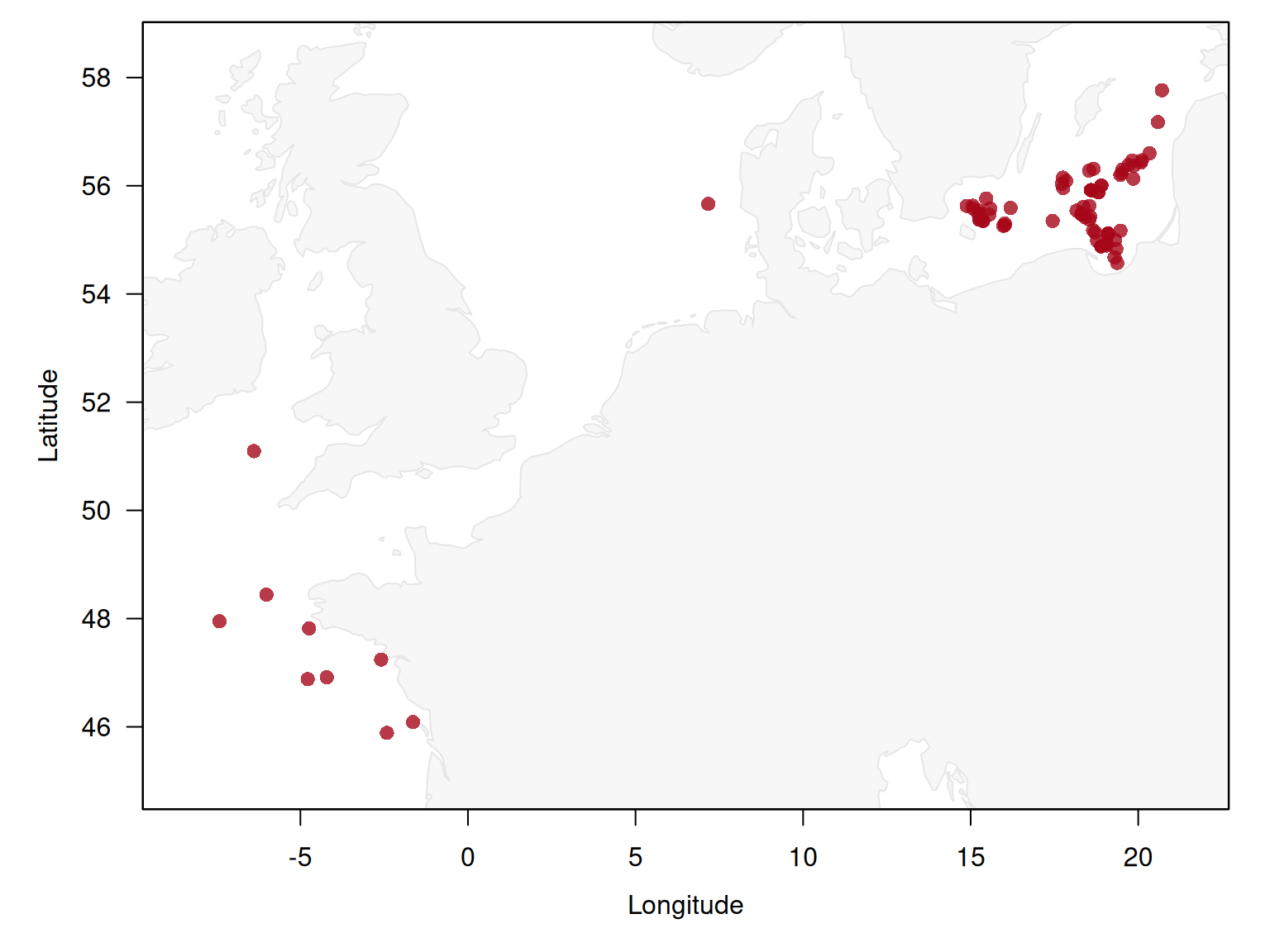

Flags concentrated in one survey, one ship or one year point at a recording convention rather than at individual bad hauls.

Spatial and temporal coverage

plot_datras_overview(surv, mode = "grid", metric = "count_hauls",
                     spatial_basis = "statrec")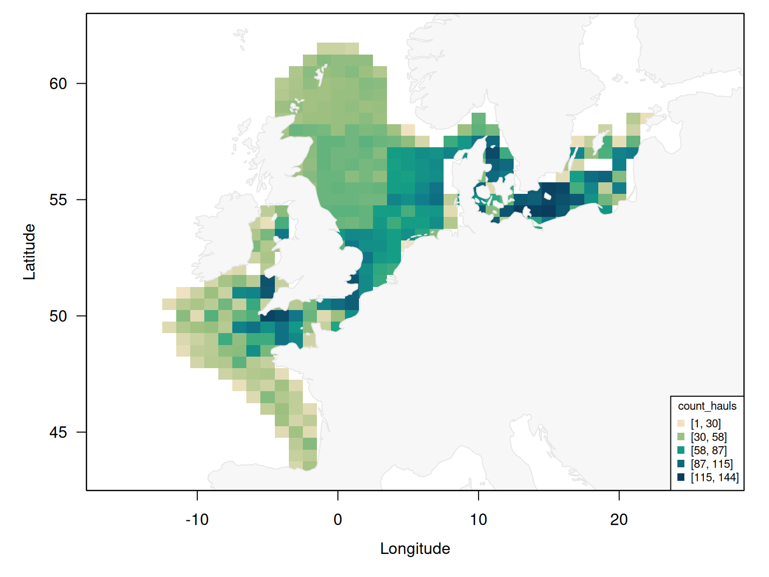

plot_datras_overview(surv, value_var = "Depth", by_survey = TRUE,
                     multi_panels = TRUE)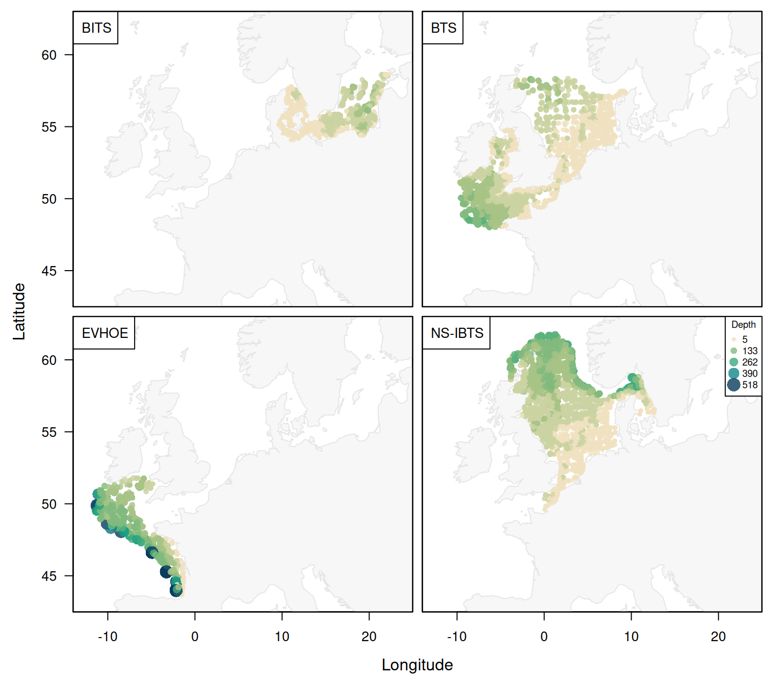

Mapping a covariate such as depth by survey exposes both spatial gaps and values that are locally implausible even though they pass a global range check.

Length and composition sanity

plot_length_distribution(plaice, log_scale = TRUE)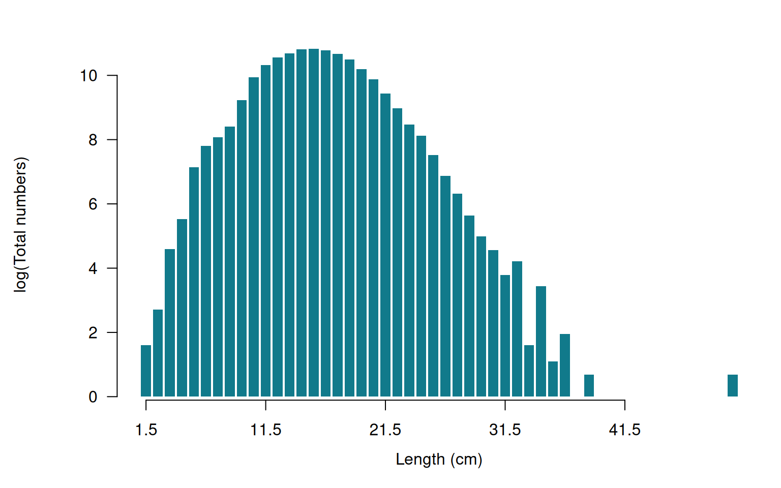

A spectrum with isolated spikes at round numbers, or a long thin tail beyond the empirical maximum length, indicates unit or transcription problems.

comp <- add_numbers_at_length(surv)
comp <- add_total_numbers_by_haul(comp, length_cuts = c(0, 15, 30, 50, Inf))
plot_species_composition(comp, beside = FALSE, legend_ncol = 2)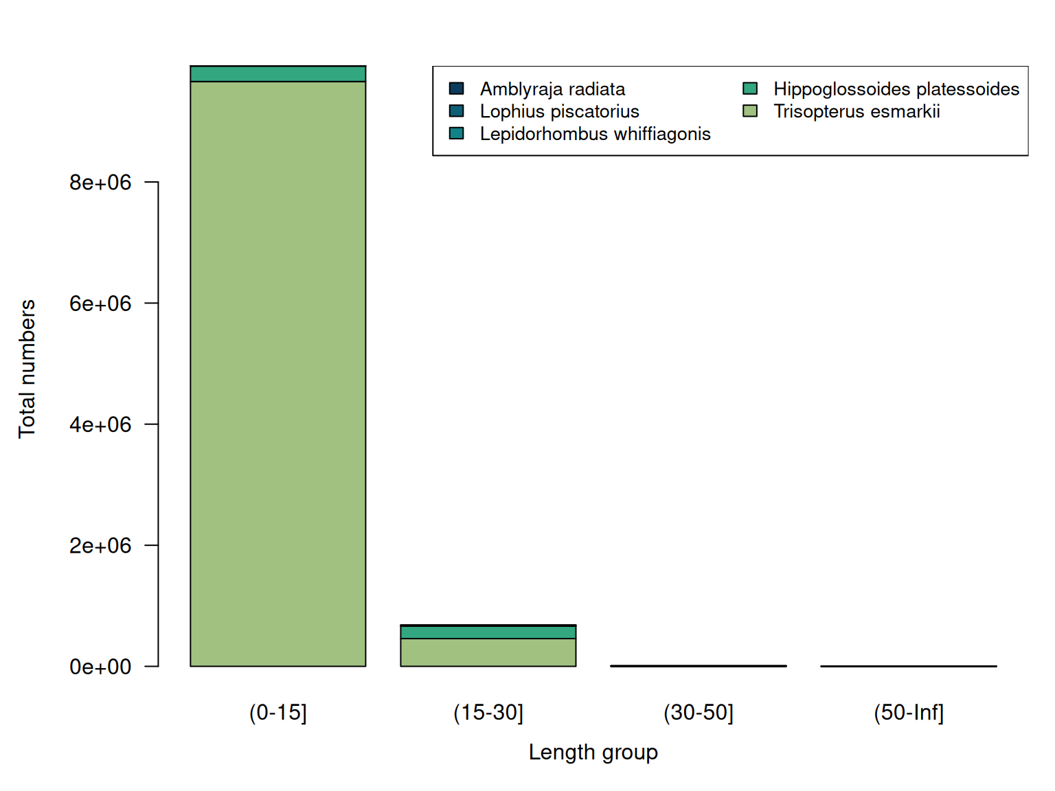

Composition by length group exposes problems a total does not: a species that appears only in one length group, or a length group dominated by a single species across every survey, is usually a binning or identification artefact rather than ecology.

Spatial attribution

surv_area <- add_ices_areas(surv)
#> Matched 12700 of 12725 hauls to ICES areas (25 unmatched -> NA)

## Adds Area_Full, Area_27 and Ecoregion to HH
head(sort(table(surv_area[["HH"]]$Area_27), decreasing = TRUE))
#> 
#>    4.b    4.a 3.d.25    7.e    4.c 3.d.24 
#>   2826   1488   1018    803    776    611

## Hauls that could not be attributed
sum(is.na(surv_area[["HH"]]$Area_27))
#> [1] 1243

The function reports how many hauls it matched. Hauls that cannot be matched to an ICES area usually have a coordinate problem that range checks alone will not catch.

Recording and verifying the extraction

DATRAS is revised continuously. ICES does not only append new observations, it also corrects haul metadata, re-ages samples and reclassifies species, so a script that is unchanged can produce different numbers a year later. Nothing in the exchange file carries a version number, which makes this hard to notice.

The ICES calculation date

There is, however, one field that acts as an upstream version stamp: DateofCalculation, recording when ICES last recalculated a block of records. It is constant per survey, year and quarter and identical across HH, HL and CA. Because it is set by ICES rather than by us, it can be compared between two extractions made at any time.

Coverage is good but not complete. In a full local copy of DATRAS, 918 of 970 survey-year-quarters carry a date. Most of the gaps are historical, but a handful are not: SP-NORTH quarter 3 and SP-PORC quarter 4 are missing the field for several years in the 2000s. Where the date is absent, an upstream revision cannot be detected this way, and only the file checksum will show that something changed.

extraction() reads it out, together with everything else known about where the data came from:

extraction(mini)[c("survey", "year", "quarter", "date_of_calculation")]
#>     survey year quarter date_of_calculation
#> 1     BITS 2015       1          2020-04-08
#> 2     BITS 2015       4          2022-04-22
#> 3     BITS 2016       1          2024-08-09
#> 4     BITS 2016       4          2024-08-14
#> 5     BITS 2017       1          2024-08-14
#> 6     BITS 2017       4          2024-08-15
#> 7     BITS 2018       1          2021-04-28
#> 8     BITS 2018       4          2024-08-15
#> 9     BITS 2019       1          2024-08-15
#> 10    BITS 2019       4          2022-04-27
#> 11    BITS 2020       1          2022-04-07
#> 12    BITS 2020       4          2024-07-12
#> 13     BTS 2015       1          2020-05-25
#> 14     BTS 2015       3          2022-04-11
#> 15     BTS 2016       1          2020-05-25
#> 16     BTS 2016       3          2022-04-11
#> 17     BTS 2017       1          2020-05-25
#> 18     BTS 2017       3          2022-04-11
#> 19     BTS 2018       1          2020-05-25
#> 20     BTS 2018       3          2021-12-09
#> 21     BTS 2019       1          2020-05-25
#> 22     BTS 2019       3          2021-12-09
#> 23     BTS 2020       1          2021-03-04
#> 24     BTS 2020       3          2021-12-09
#> 25   EVHOE 2015       4          2016-04-16
#> 26   EVHOE 2016       4          2018-05-07
#> 27   EVHOE 2017       4          2018-04-23
#> 28   EVHOE 2018       4          2019-03-05
#> 29   EVHOE 2019       4          2020-02-19
#> 30   EVHOE 2020       4          2021-02-22
#> 31 NS-IBTS 2015       1          2021-06-07
#> 32 NS-IBTS 2015       2          2019-03-07
#> 33 NS-IBTS 2015       3          2017-03-16
#> 34 NS-IBTS 2016       1          2017-09-14
#> 35 NS-IBTS 2016       3          2023-03-22
#> 36 NS-IBTS 2017       1          2023-03-22
#> 37 NS-IBTS 2017       3          2021-10-29
#> 38 NS-IBTS 2018       1          2022-07-12
#> 39 NS-IBTS 2018       3          2022-01-25
#> 40 NS-IBTS 2019       1          2021-10-04
#> 41 NS-IBTS 2019       3          2022-01-25
#> 42 NS-IBTS 2020       1          2022-01-25
#> 43 NS-IBTS 2020       3          2022-04-08

The bundled mini data set was created long before this information was recorded, yet the table is still populated: the survey, year, quarter and calculation date are reconstructed from the data themselves whenever no explicit record is available. The same is true of any archive downloaded with an earlier version of the package.

Reading this table is already informative. Above, NS-IBTS quarter 1 was recalculated for all six years on 2026-06-25, long after most other blocks, so results using it may differ from an analysis run before that date.

What else is recorded

When data are downloaded with download_datras(), the remaining columns are filled in as well:

extracted, source and endpoint: when the data were retrieved and from where,
file, payload_hash, zip_hash and algo: which archive file the records came from and its checksum,
read: when the archive was read into R,
datrasextra, datras, icesdatras and r_version: the software that produced the object.

The record follows the object through the pipeline, so a derived product can always be traced back to the extraction it came from:

nrow(extraction(check_outliers(clean_datras(mini, verbose = FALSE),
                               action = "remove", verbose = FALSE)))
#> [1] 43

It is also reconciled with the data actually present, so subsetting narrows it rather than leaving stale entries behind:

extraction(subset(mini, Year == 2020 & Quarter == 1))[1:4]
#>    survey year quarter date_of_calculation
#> 1    BITS 2020       1          2022-04-07
#> 2     BTS 2020       1          2021-03-04
#> 3 NS-IBTS 2020       1          2022-01-25

survey and extracted are exactly the two fields the ICES citation format requires, so the record can be formatted straight into a data citation:

e <- extraction(x)
sprintf("ICES Database of Trawl Surveys (DATRAS), Extraction %s of %s. ICES, Copenhagen",
        format(max(e$extracted), "%d %B %Y"),
        paste(unique(e$survey), collapse = ", "))

Verifying a snapshot

write_manifest() describes a whole archive in one file, DATRAS_manifest.csv, holding a checksum and calculation date for every survey-year-quarter it contains. download_datras() maintains it automatically, and it can be built for any directory of exchange files, including one a colleague sent you:

write_manifest("data/datras")

verify_extraction() then re-reads the archive and compares:

verify_extraction("data/datras")

Each entry comes back as ok, changed, revised, missing or new. The distinction between the middle two is the point of the exercise:

changed means the file contents differ but the ICES calculation date is the same. That is a local problem, typically a partial download or a corrupted copy.
revised means ICES has recalculated the data since the manifest was written. Results derived from the old copy will not reproduce against the new one, and this is otherwise invisible.

Two people can also compare manifests directly to confirm they hold identical data without either of them hosting anything.

Note that the checksum is taken over the exchange file inside the zip archive, not over the archive itself. utils::zip() stores the modification time of the file it compresses, so writing identical data twice produces different archives but the same payload checksum. Only the payload checksum answers “is this the same data”.

How old are the bundled lookup tables?

The same question applies to the reference data the package ships with. species_info, survey_info and the internal ICES-area lookup are snapshots of external sources – WoRMS, FishBase, the ICES web services – taken at a particular time, so an analysis can depend on how old they are. reference_tables() says:

reference_tables()[c("table", "kind", "rows", "generated", "status")]
#>                  table     kind   rows  generated status
#> 1        spawning_info exported   1023 2026-09-15     ok
#> 2         species_info exported   2064 2026-09-15     ok
#> 3          survey_info exported     28 2026-10-03     ok
#> 4 survey_info_full_raw exported 144401 2026-10-03     ok
#> 5     ices_area_lookup internal   6758 2026-10-03     ok
#> 6        spread_models internal     12 2026-10-03     ok

generated is when each table entered the package, and status compares the table against the hash recorded in the package registry, so changed means a table was regenerated without its metadata being updated. The source column records what each was built from:

r <- reference_tables(check = FALSE)
r$source[r$table == "species_info"]
#> [1] "WoRMS via the worrms package; FishBase via rfishbase; DATRAS length-weight table (August 2023); functional groups from Walker et al. (2017), van Denderen et al. (2020) and Mildenberger et al. (2025)"

Taxonomy is the case where this matters most. get_aphia() and get_latin() resolve names against species_info by default, so they reflect WoRMS as of the date above rather than WoRMS today. Pass use_worrms = TRUE to query WoRMS live instead.

What this does and does not give you

This records and verifies; it does not preserve. A reader who has the extraction date and checksum still cannot obtain that exact snapshot from ICES, because the web service always serves the current state of the database. The archive written by download_datras() remains the only fixed point in the workflow, so keep it, and keep its manifest alongside it.

Between them, extraction() and reference_tables() cover both halves of the question: how old the survey data are, and how old the lookup tables applied to them are.

Further checks worth considering

The following are not built into DATRASextra, because the right treatment depends on the analysis. They are common sources of trouble.

Survey design changes over time. Gear, ship and sweep length changes create step changes in catchability that look like population signal.

with(surv[["HH"]], table(Year, Gear))
#>       Gear
#> Year   TVL TVS BT4A BT4AI BT4P BT4S BT7 BT8 GOV
#>   2015 294 227   80   108  135  191  63 155 885
#>   2016 338 249   79   107  137  188  63 159 898
#>   2017 382 244  134   102  128  128  63 133 739
#>   2018 376 241  134   104  116  116  63 157 868
#>   2019 358 230  134   108  132  132  63 144 846
#>   2020 357 250  132    32   81   81  63 147 851

Species validity codes. SpecVal in HL marks how a species record should be used, and clean_datras() does not filter on it. Code 1 is fully valid; others indicate partial or unusable records.

table(mini[["HL"]]$SpecVal, useNA = "ifany")
#> 
#>     0     1     4     6     7 
#>   383 84157     3     1     1

Mixed reporting conventions. Check DataType per survey and year, not just overall (see Stage 3).

Day and night composition. Catchability of many species differs strongly between day and night, and the day/night ratio can drift across years.

with(surv[["HH"]], table(Year, DayNight))
#>       DayNight
#> Year      D    N
#>   2015 2048   90
#>   2016 2137   81
#>   2017 1910  143
#>   2018 2024  151
#>   2019 1996  151
#>   2020 1947   47

Seasonal drift. A survey nominally in quarter 1 may drift by several weeks over a time series; timeOfYear makes that visible.

tapply(surv[["HH"]]$timeOfYear, surv[["HH"]]$Year, function(z)
  round(range(z, na.rm = TRUE), 3))
#> $`2015`
#> [1] 0.033 0.958
#> 
#> $`2016`
#> [1] 0.033 0.944
#> 
#> $`2017`
#> [1] 0.049 0.961
#> 
#> $`2018`
#> [1] 0.038 0.966
#> 
#> $`2019`
#> [1] 0.008 0.961
#> 
#> $`2020`
#> [1] 0.025 0.958

Depth against bathymetry. Recorded depth can be cross-checked against an external bathymetry raster. Systematic offsets usually indicate a unit or datum problem.

Internal catch consistency. TotalNo and CatCatchWgt in HL should be consistent with the summed HLNoAtLngt for the same haul, species and category. Large discrepancies indicate sub-sampling information that has not been applied consistently.

Age data plausibility. Length-at-age should be monotone on average and its spread should not collapse or explode at the oldest ages. Also check ALK coverage: ages sampled in too few hauls give unstable keys.

Duplicate biological records. Exact duplicate rows within a haul and species in HL or CA are worth counting, since they inflate abundance without tripping any range check.

Reference data coverage. add_species_info() joins the bundled species table; check which species come back without length-weight parameters or maximum length, because those silently degrade any weight-based calculation.

info <- add_species_info(surv, vars = c("maxL", "a", "b"), verbose = FALSE)

## TRUE means the species has no length-weight parameters in species_info
with(info[["HL"]], tapply(is.na(a), Species, all))
#>            Amblyraja radiata Hippoglossoides platessoides 
#>                        FALSE                        FALSE 
#>   Lepidorhombus whiffiagonis          Lophius piscatorius 
#>                        FALSE                        FALSE 
#>         Trisopterus esmarkii 
#>                        FALSE

All five species in mini are covered. In a full survey extract, with several hundred taxa, a handful typically are not.

A reproducible recipe

Putting the stages together:

## 1-2. Download once, then read from the archive
download_datras(path = "data/datras", surveys = "NS-IBTS", years = 2015:2023)
verify_extraction("data/datras")                    # confirm the snapshot
x <- read_datras("data/datras", surveys = "NS-IBTS", years = 2015:2023)

## Audit the read before anything is filtered
extraction(x)
sum(is.na(x[["CA"]]$haul.id))
table(x[["HH"]]$DataType)
get_accuracy_cm(x)

## 3. Clean, with a full account of what is removed
x <- clean_datras(x, explain_codes = TRUE)

## 4. Check, without removing anything yet
x <- check_outliers(x, pct = TRUE)
report <- attr(x, "outlier_report")

## 5. Look at the flags before deciding
plot_datras_overview(subset(x, haul.id %in% attr(x, "outlier_hauls_invalid")))

## 6. Remove only what you have decided is wrong
x <- check_outliers(x, action = "remove", verbose = FALSE)

## 7. Derived variables, with their own diagnostics
x <- add_swept_area(x, full_report = TRUE)
x <- add_numbers_at_length(x)
x <- add_total_numbers_by_haul(x)

summary(x)

Keep extraction(x) with the results. It is what lets you, or someone else, establish later whether a difference in the numbers comes from the code or from the data.

Summary

Stage	Automatic steps	Under your control
Download	code renaming, `-9` to `NA`, strict haul matching, exchange archiving	`surveys`, `years`, `download_hl`, `download_ca`, `include_flagged`, `overwrite`, `timeout`
Read	corrupt-file check, empty-file exclusion, duplicate haul removal, type-safe combining	`strict`, `min_file_size`, `prune`, `drop_hl`, `drop_ca`, `surveys`, `years`, `ncores`
Derived variables	`haul.id`, `LngtCm`, `Species`, `Count`, `lon`/`lat`, `abstime`, `Roundfish`, zero-catch treatment	length binning via `cm_breaks` / `by`
Cleaning	`HaulVal` and `StdSpecRecCode` filters	`verbose`, `explain_codes`, `impute_missing_depth`, `correct_species`, `aphias`, `years`, `quarters`, `gears`, `do_fishglob`
Checks	none by default	`check_outliers()` (`strict`, `pct`, `pct_*`, `vars`, `action`, `remove_extremes`), `check_lengths()`, `check_weights()`, `add_swept_area()`
Extraction record	attached on read, propagated through the pipeline, reconciled with the data present	`extraction()`, `write_manifest()`, `read_manifest()`, `verify_extraction()`

Nothing in the automatic column is hidden: the download and read stages print what they do, clean_datras() reports the data before filtering, and every check writes its findings to an attribute you can inspect. Where a step cannot be switched off by argument, it is a plain subset() call that can be replaced with a rule of your own.

References

ICES DATRAS database: https://datras.ices.dk
ICES vocabularies for HaulVal, StdSpecRecCode and BySpecRecCode: https://vocab.ices.dk
vignette("datrasextra-tutorial") for the basic workflow
vignette("articles/fishglob") for the FishGlob pipeline

Overview of the pipeline

Stage 1: Download

Which surveys and years are requested

Harmonisation applied on download

What gets archived

Stage 2: Reading data into R

Parsing and file-level checks

Matching biological records to hauls: the strict argument

Combining survey-year files

Stage 3: Variables created while reading

Haul identifier

Length in centimetres

Species names

Raised catch numbers

Time and position

Hauls without catch records

The ICES calculation date

Type coercions to be aware of

Stage 4: Cleaning with clean_datras()

Filter 1: haul validity

Filter 2: standard species recording

Optional: imputing missing depths

Optional: harmonising species

Optional: subsetting

Modifying or omitting steps

Stage 5: Quality-control checks

check_outliers()

Rule-based checks

Percentile checks

Running the checks

Acting on the results

check_lengths()

check_weights()

add_swept_area()

Stage 6: Inspecting the result

Tabular summaries

Mapping the flagged hauls

Spatial and temporal coverage

Length and composition sanity

Spatial attribution

Recording and verifying the extraction

The ICES calculation date

What else is recorded

Verifying a snapshot

How old are the bundled lookup tables?

What this does and does not give you

Further checks worth considering

A reproducible recipe

Summary

References

Matching biological records to hauls: the `strict` argument

Stage 4: Cleaning with `clean_datras()`

`check_outliers()`

`check_lengths()`

`check_weights()`

`add_swept_area()`