Processing ICES DATRAS Data for FishGlob • DATRASextra

Background

The FishGlob database is a global compilation of standardized scientific trawl survey data used to study large-scale patterns in marine fish biodiversity and community structure.

FishGlob harmonizes data from multiple regional monitoring programs by standardizing:

taxonomic information
sampling effort
catch metrics (abundance and biomass per unit area)

The dataset integrates numerous long-term fisheries-independent surveys, including several surveys available through the ICES DATRAS database.

ICES DATRAS (Database of Trawl Surveys) provides access to standardized survey data collected in European seas, including haul-level sampling information (HH), length distributions (HL), and individual data (CA).

The DATRASextra package provides tools to process raw DATRAS survey data and generate outputs that are compatible with the FishGlob data structure.

This vignette demonstrates a workflow to:

download DATRAS survey data
harmonize and clean_datras raw survey tables
standardize species taxonomy
estimate swept area and biomass
generate FishGlob-compatible datasets

The workflow can be applied to a single species or to multiple species. For illustration, this vignette uses mini.

data("mini_fishglob", package = "DATRASextra")

an example dataset containing 6 species across 4 surveys (BITS, BTS, EVHOE, NS-IBTS):

Amblyraja radiata, Hippoglossoides platessoides, Trisopterus esmarkii, Lophius piscatorius, Lepidorhombus whiffiagonis

References

Maureaud, A., et al. (2021) FISHGLOB_data: an integrated dataset of fish biodiversity sampled with scientific bottom-trawl surveys. Sci Data 11, 24 (2024). https://doi.org/10.1038/s41597-023-02866-w

ICES Database on Trawl Surveys (DATRAS), ICES, Copenhagen, Denmark. https://datras.ices.dk

Libraries

library(DATRASextra)

## Loading required package: DATRAS

library(ggplot2)
library(dplyr)

## 
## Attaching package: 'dplyr'

## The following objects are masked from 'package:stats':
## 
##     filter, lag

## The following objects are masked from 'package:base':
## 
##     intersect, setdiff, setequal, union

Load the dataset

data(mini_fishglob)

Clean the dataset

The clean_fishglob() function harmonizes the raw DATRAS tables and prepares them for processing. Species names and identifiers are standardized using WoRMS taxonomy with correct_species() This step ensures:

consistent scientific names
valid AphiaID identifiers
standardized taxonomic classification

dat <- clean_fishglob(mini_fishglob)

Reduce dataset size

The raw dataset contains many variables that are not required for the FishGlob output.

The prune_fishglob() function removes unnecessary columns to reduce memory usage and improve processing speed.

dat <- prune_fishglob(dat)

Compute swept area

Catch per unit area requires an estimate of the area swept by each haul.

The function below:

calculates swept area when gear information is available
imputes missing values when necessary

dat <- add_swept_area_fishglob(dat)

Estimate biomass

FishGlob reports both numbers and biomass.

The add_total_weight_by_haul_fishglob() function converts length data to weight using species-specific length–weight relationships.

dat <- add_total_weight_by_haul_fishglob(dat)

Format the FishGlob output

Finally, the dataset is formatted to match the FishGlob data structure.

datras <- as_fishglob(dat)

head(datras)

##     survey      source timestamp                          haul_id
## 2     BITS DATRAS ICES   2026-05  BITS:2015:1:DE:06SL:TVS:22004:7
## 4     BITS DATRAS ICES   2026-05  BITS:2015:1:DE:06SL:TVS:22007:8
## 44    BITS DATRAS ICES   2026-05 BITS:2015:1:DE:06SL:TVS:24212:15
## 110   BITS DATRAS ICES   2026-05      BITS:2015:1:DK:26HI:TVS:1:1
## 111   BITS DATRAS ICES   2026-05    BITS:2015:1:DK:26HI:TVS:10:10
## 112   BITS DATRAS ICES   2026-05    BITS:2015:1:DK:26HI:TVS:10:10
##             country sub_area continent stat_rec station stratum year month day
## 2   multi-countries     <NA>    europe     37G0    <NA>    <NA> 2015     2  25
## 4   multi-countries     <NA>    europe     37G1    <NA>    <NA> 2015     2  26
## 44  multi-countries     <NA>    europe     38G3    <NA>    <NA> 2015     2  28
## 110 multi-countries     <NA>    europe     43G0    <NA>    <NA> 2015     2  24
## 111 multi-countries     <NA>    europe     41G2    <NA>    <NA> 2015     2  27
## 112 multi-countries     <NA>    europe     41G2    <NA>    <NA> 2015     2  27
##     quarter latitude longitude haul_dur area_swept gear depth     num num_cpue
## 2         1  54.4427   10.6547      0.5 0.07697517  TVS    19   1.000    2.000
## 4         1  54.4513   11.3738      0.5 0.08368994  TVS    20   1.000    2.000
## 44        1  54.9908   13.3447      0.5 0.09056468  TVS    47   1.000    2.000
## 110       1  57.4721   10.6695      0.5 0.07173646  TVS    26  90.573  181.146
## 111       1  56.1206   12.4688      0.5 0.06509888  TVS    26   1.000    2.000
## 112       1  56.1206   12.4688      0.5 0.06509888  TVS    26 118.635  237.270
##       num_cpua        wgt   wgt_cpue   wgt_cpua verbatim_name verbatim_aphia_id
## 2     12.99120 0.01259440  0.0251888  0.1636164          <NA>                NA
## 4     11.94887 0.06313433  0.1262687  0.7543837          <NA>                NA
## 44    11.04183 0.05369922  0.1073984  0.5929377          <NA>                NA
## 110 1262.57974 2.06026668  4.1205334 28.7199381          <NA>                NA
## 111   15.36125 2.93347786  5.8669557 45.0618790          <NA>                NA
## 112 1822.38158 5.13663026 10.2732605 78.9050479          <NA>                NA
##                    accepted_name aphia_id          class             order
## 2   Hippoglossoides platessoides   127137      Teleostei Pleuronectiformes
## 4   Hippoglossoides platessoides   127137      Teleostei Pleuronectiformes
## 44  Hippoglossoides platessoides   127137      Teleostei Pleuronectiformes
## 110 Hippoglossoides platessoides   127137      Teleostei Pleuronectiformes
## 111            Amblyraja radiata   105865 Elasmobranchii        Rajiformes
## 112 Hippoglossoides platessoides   127137      Teleostei Pleuronectiformes
##             family           genus    rank survey_unit
## 2   Pleuronectidae Hippoglossoides Species      BITS-1
## 4   Pleuronectidae Hippoglossoides Species      BITS-1
## 44  Pleuronectidae Hippoglossoides Species      BITS-1
## 110 Pleuronectidae Hippoglossoides Species      BITS-1
## 111        Rajidae       Amblyraja Species      BITS-1
## 112 Pleuronectidae Hippoglossoides Species      BITS-1

Compare it with Fishglob

Download FishGlob

# load survey data
fishglob_url <- "https://github.com/AquaAuma/FishGlob_data/raw/d71dfa03c2912b4e9d9cd10412ae2af52ba56ae5/outputs/Compiled_data/FishGlob_public_std_clean.RData" # stick with this version
options(timeout = 300) # increase timeout to 5 minutes
load(url(fishglob_url))
fishglob <- data

Get the surveys in common

common_surveys <- intersect(fishglob$survey, datras$survey)

fishglob_common <- fishglob[fishglob$survey %in% common_surveys, ]
datras_common <- datras[datras$survey %in% common_surveys, ]

fishglob_common$haul_id <- gsub(" ", ":", fishglob_common$haul_id) # use our haul format

# get common haul ids
common_haul_ids <- intersect(fishglob_common$haul_id, datras_common$haul_id)

# fishglob
fishglob_agg <- fishglob_common %>% filter(haul_id %in% common_haul_ids) %>%
  group_by(haul_id, accepted_name, survey) %>%
  summarise(wgt_cpua = sum(wgt_cpua, na.rm = TRUE), num = sum(num, na.rm = TRUE), .groups = "drop")

# datras_extra
datras_agg <- datras_common %>% filter(haul_id %in% common_haul_ids) %>%
  group_by(haul_id, accepted_name, survey) %>%
  summarise(wgt_cpua = sum(wgt_cpua, na.rm = TRUE), num = sum(num, na.rm = TRUE), .groups = "drop")

merged_agg <- merge(
  fishglob_agg,
  datras_agg,
  by = c("survey","haul_id", "accepted_name"),
  suffixes = c("_fishglob", "_datras")
)

am_dab <- merged_agg %>%
  filter(accepted_name == "Hippoglossoides platessoides") # compare american dab as example

Plot it

ggplot(am_dab, aes(x = num_fishglob,
                   y = num_datras)) +

  # Points
  geom_point(alpha = 0.6, size = 2) +
  geom_abline(slope = 1, intercept = 0,
              color = "red", linewidth = 1) +
  labs(
    x = "FishGlob numbers",
    y = "DATRASextra numbers",
    title = "Comparison of num per haul by survey for American dab"
  ) +
  facet_wrap(~ survey, scales = "free")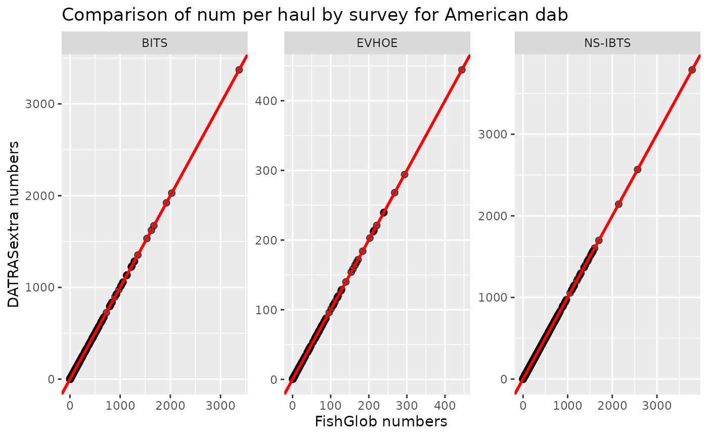

ggplot(am_dab, aes(x = wgt_cpua_fishglob,
                   y = wgt_cpua_datras)) +

  # Points
  geom_point(alpha = 0.6, size = 2) +
  geom_abline(slope = 1, intercept = 0,
              color = "red", linewidth = 1) +
  labs(
    x = "FishGlob kg/km2",
    y = "DATRASextra kg/km2",
    title = "Comparison of wgt_cpua per haul by survey for cod"
  ) +

  facet_wrap(~ survey, scales = "free")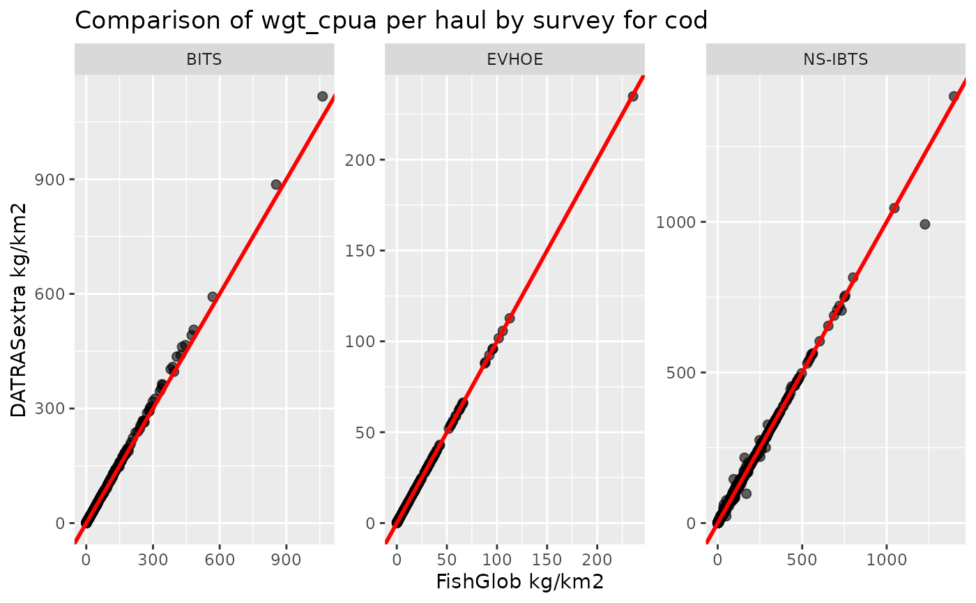

As you can see there are small differences in densities due to sligtly different swept are imputation methods.

Downloading the FishGlob DATRAS surveys

The previous example used a small dataset to keep the vignette lightweight. To reproduce the DATRAS part of the FishGlob dataset, the full set of surveys used in FishGlob can be downloaded like this:

library(DATRASextra)

surveys <- c("NS-IBTS", "EVHOE", "SWC-IBTS", "BITS", "IE-IGFS",
             "FR-CGFS", "NIGFS", "ROCKALL", "PT-IBTS",
             "SP-NORTH", "SP-ARSA", "SP-PORC")

# create temporary directory
tmp <- tempdir()

# download survey data
download_datras(surveys = surveys, dir = tmp)

# read raw DATRAS tables
raw <- read_datras(file.path(tmp, surveys))

Downloading and processing these surveys take some time, as they include multiple decades of trawl survey data.