Plotting DATRAS overviews • DATRASextra

Overview

This vignette demonstrates the unified plotting function plot_datras_overview(). The function allows to generate a quick overview of all haul locations in DATRAS or number of hauls per ICES Statistical Rectangle, but also allows to generate more complicated maps of any variables (and offset variable) by haul location in a point plot or gridded plot of a specific data set. Specifically, the function supports:

point maps (mode = "points")
gridded maps (mode = "grid")
multiple grid metrics (presence, count_hauls, count_surveys, sum, mean)
grouping and faceting (by_survey, by_gear, by_quarter, multi_panels)
raw or StatRec spatial basis (spatial_basis = "raw" or "statrec")
value/offset/transform workflows for quantitative overlays

Load the package with:

library(DATRASextra)

Quick Start

If no object is supplied (x = NULL), the function uses package survey overview data, which contains all surveys and hauls in DATRAS:

plot_datras_overview()

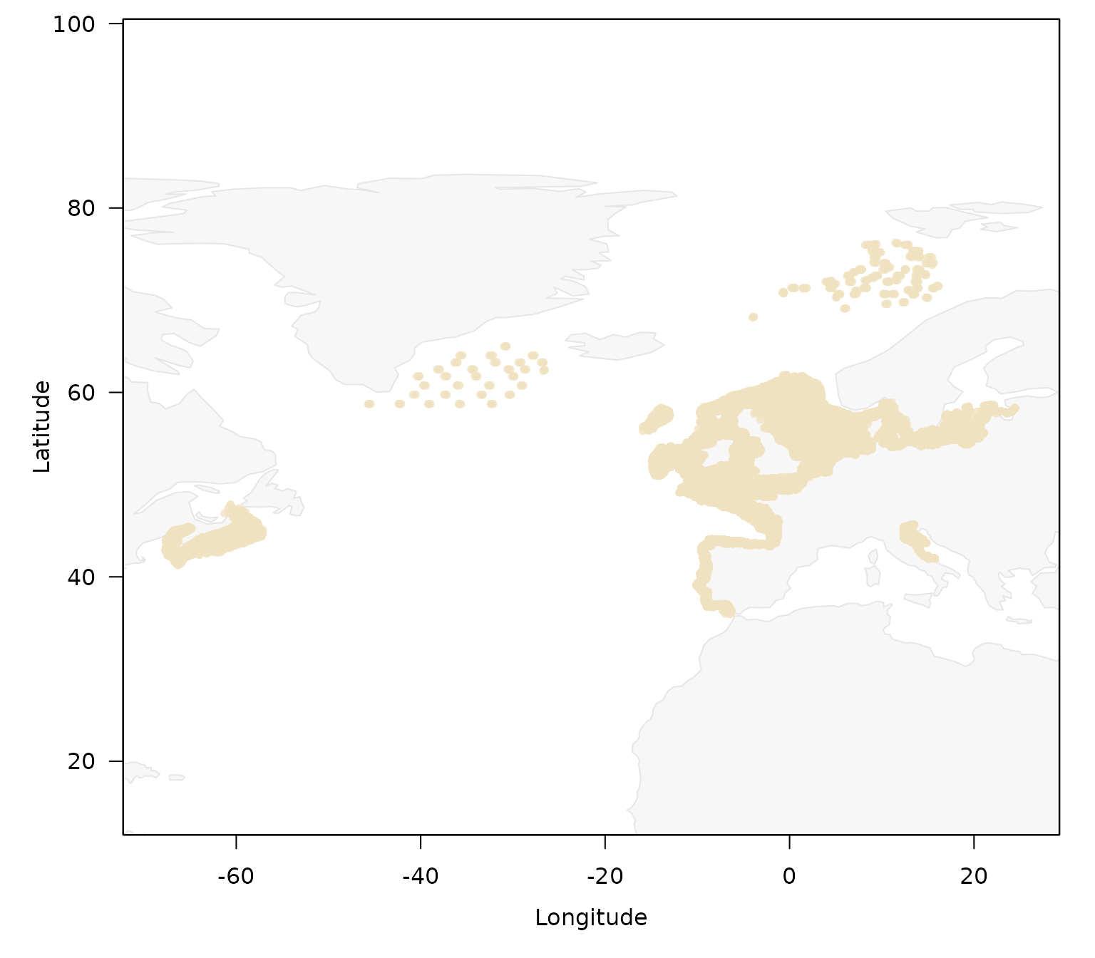
To get an overview over the surveys:

plot_datras_overview(by_survey = TRUE)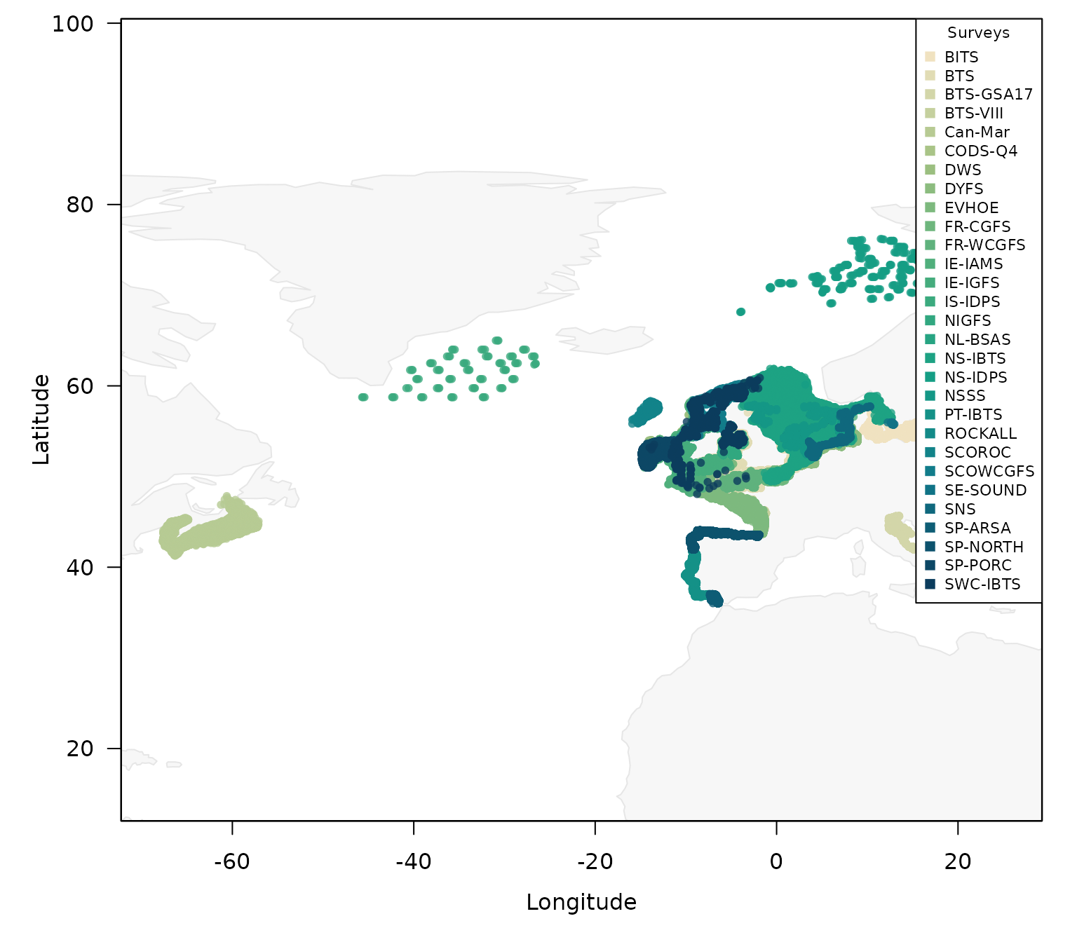

If the legend is in the way, the multiple different control arguments can be used to place and modify the legend:

plot_datras_overview(by_survey = TRUE,
                     legend_ncol = 6,
                     legend_pos = "bottom",
                     legend_cex = 0.8)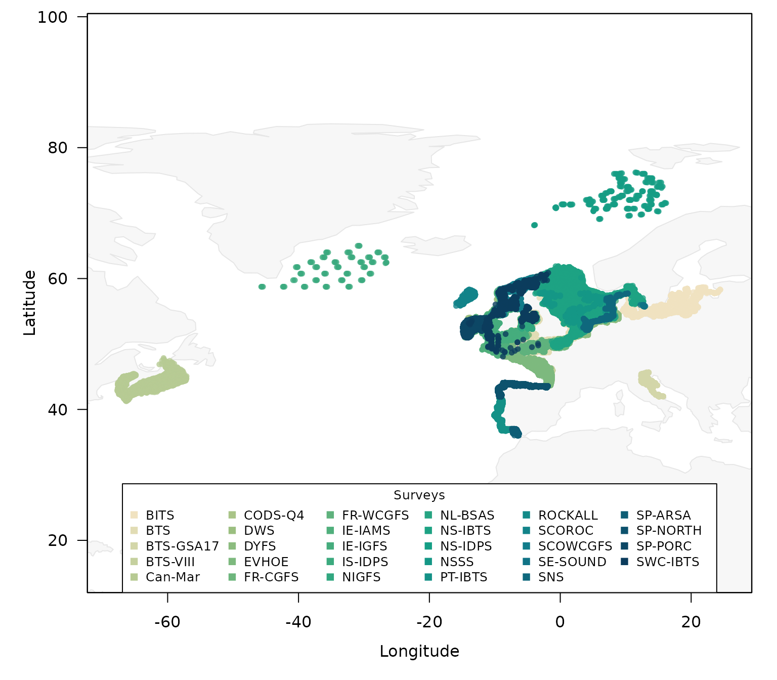

With so many surveys and repeating colours, it might be easier to plot the surveys in separate panels:

plot_datras_overview(by_survey = TRUE,
                     multi_panels = TRUE)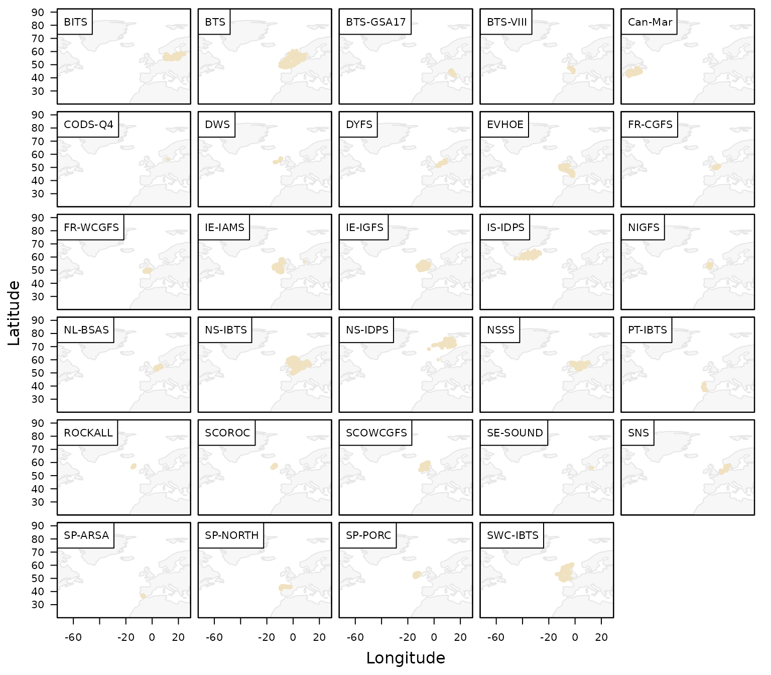

Besides the general overview over all surveys, the function also allows to create a visual overview of a specific data set, using for example the mini data set of DATRASextra:

plot_datras_overview(mini)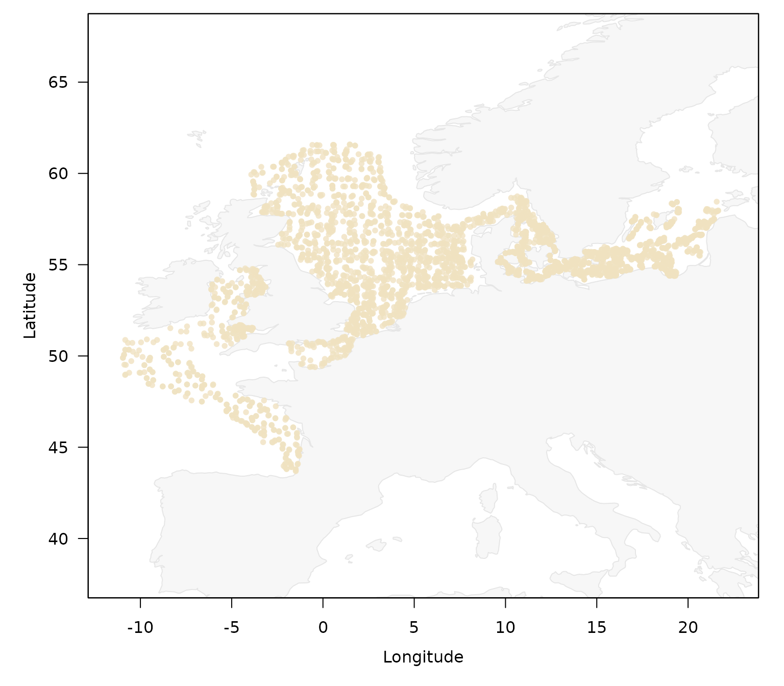

Aggregate by

Besides surveys, the function allows to quickly create a comparison between gears:

plot_datras_overview(mini, by_gear = TRUE)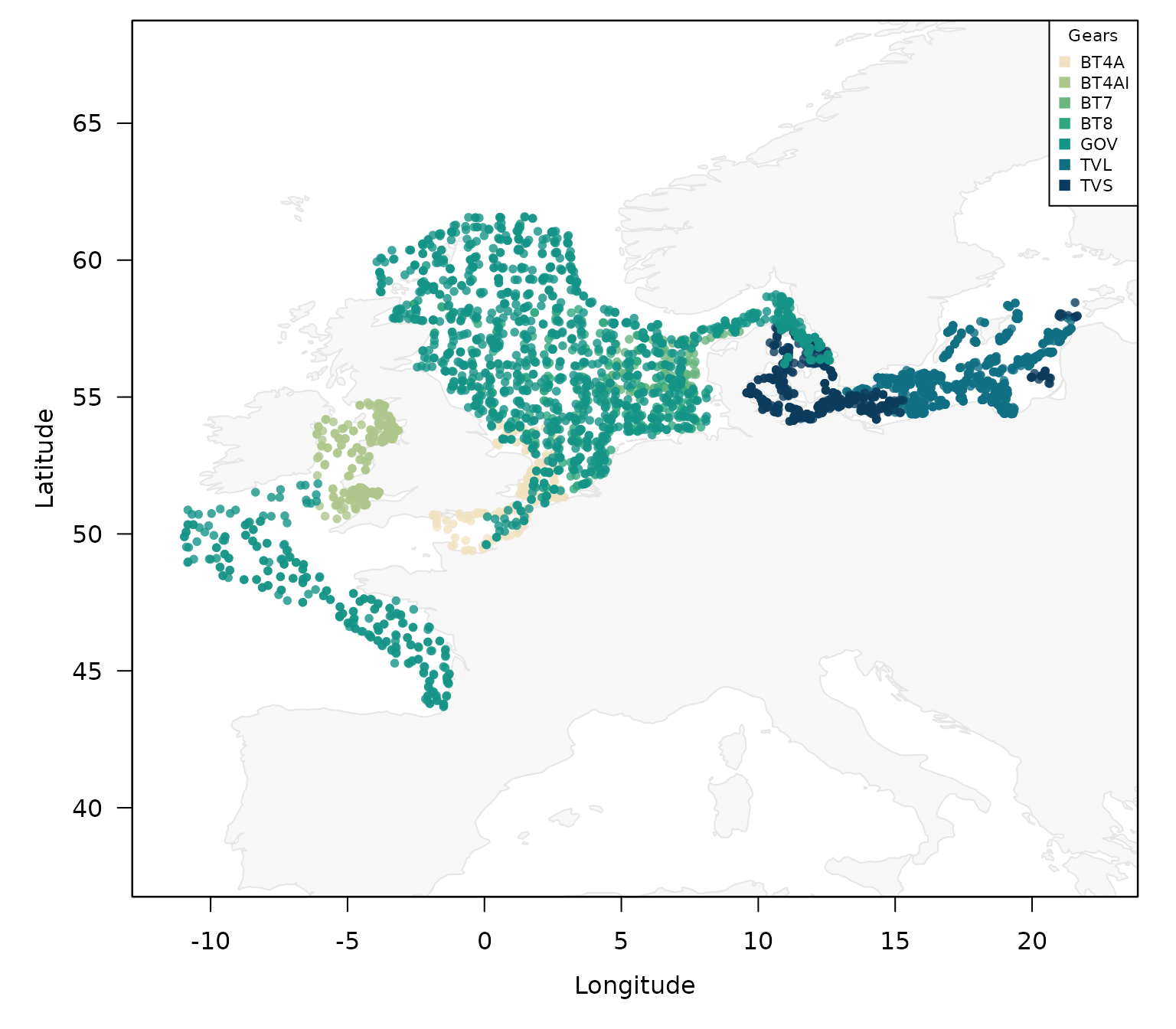

by quarter:

plot_datras_overview(mini, by_quarter = TRUE)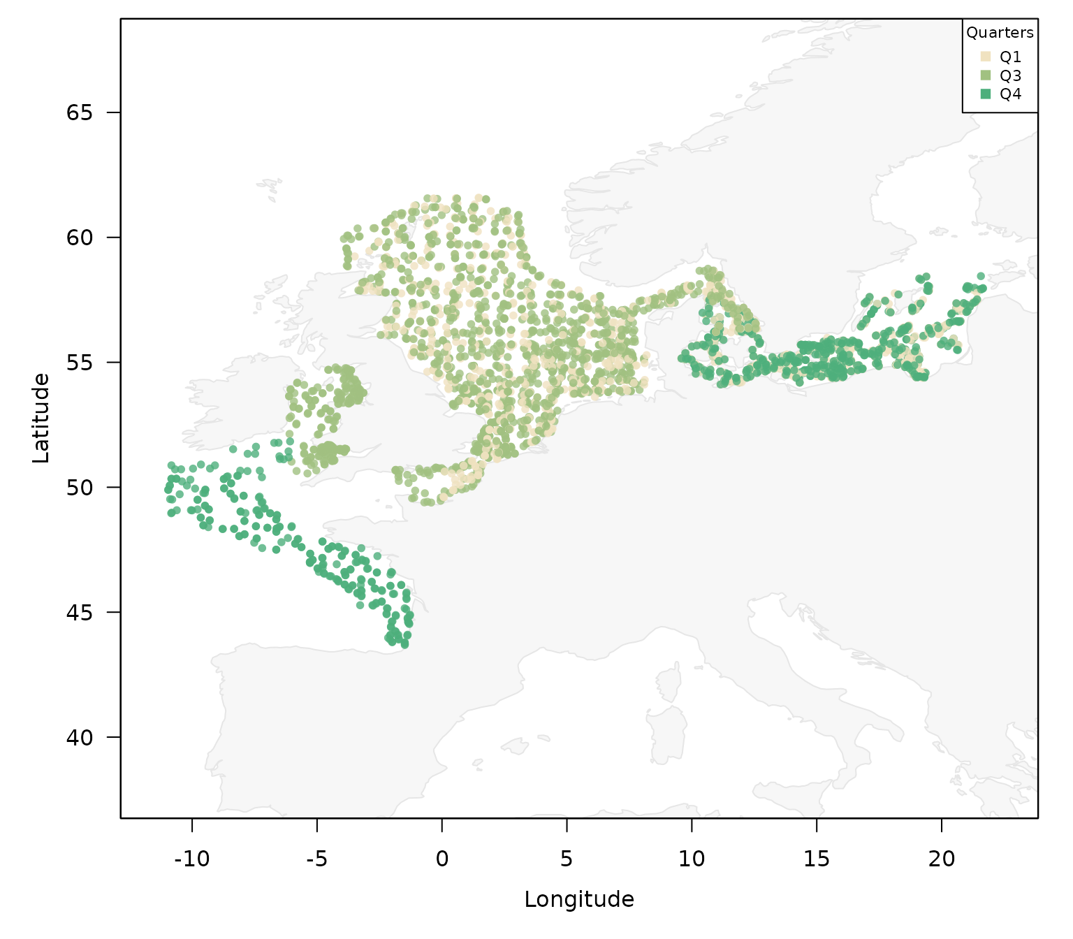

by year:

plot_datras_overview(mini, by_year = TRUE)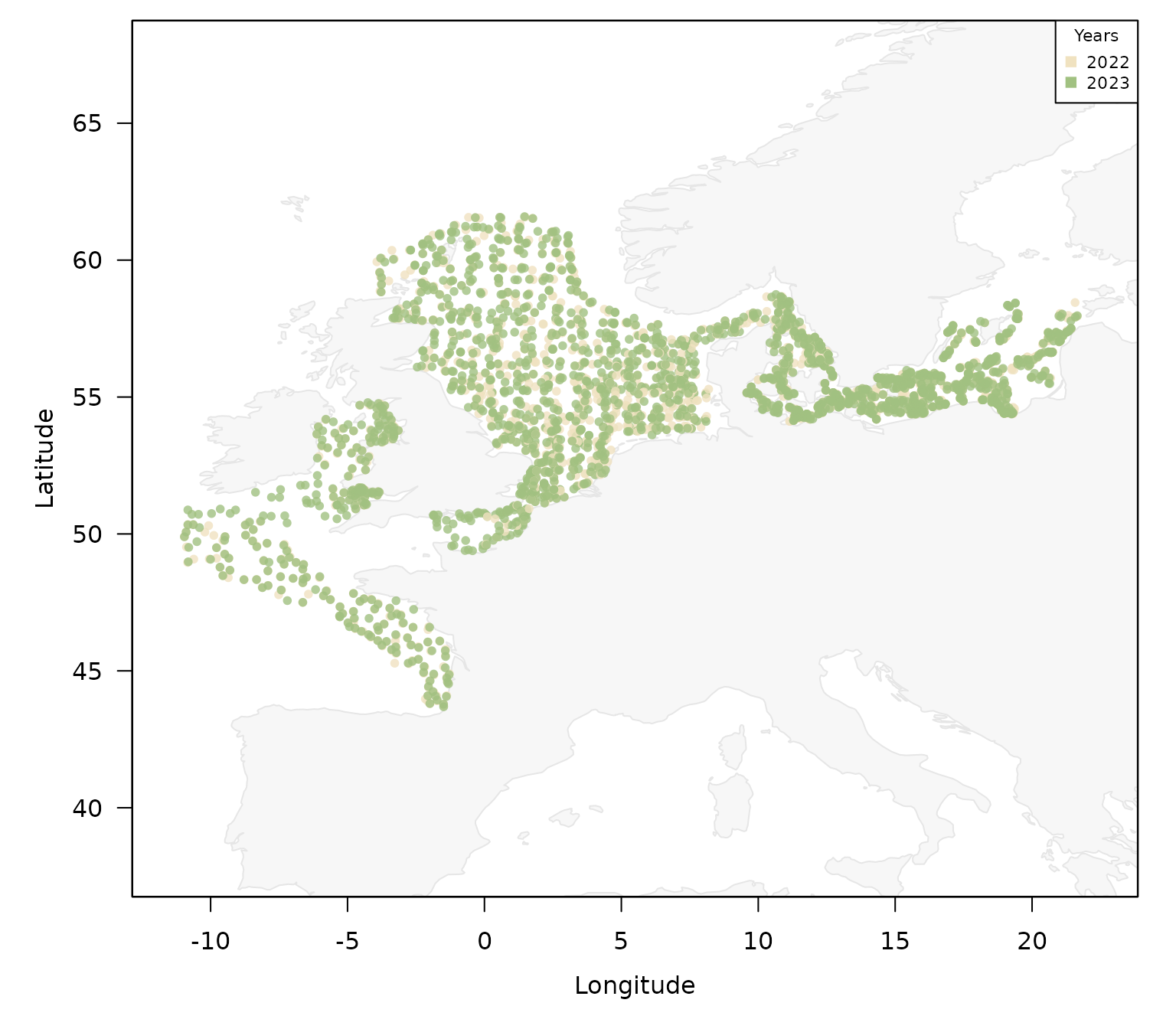

or day and night:

plot_datras_overview(mini, by_daynight = TRUE)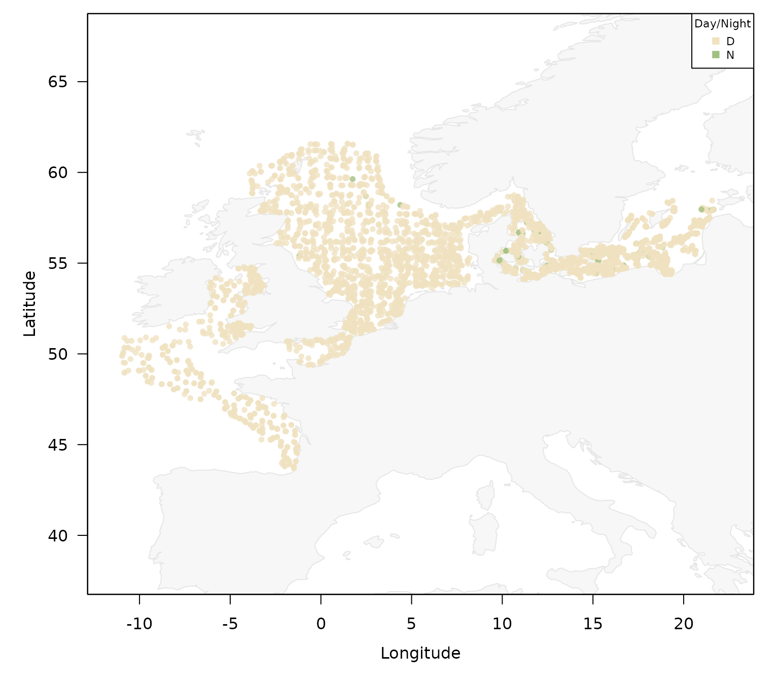

or any combination of them:

plot_datras_overview(mini,
                     by_gear = TRUE,
                     by_survey = TRUE)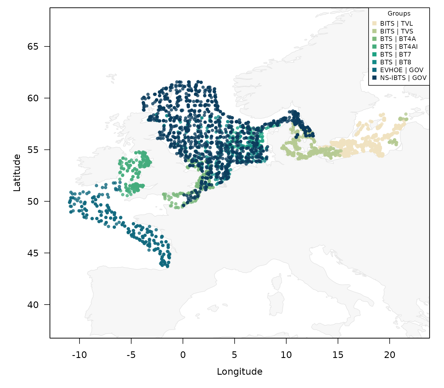

setting the multi_panel argument to TRUE avoids the overlap and might help interpretation:

plot_datras_overview(mini, by_gear = TRUE,
                     by_survey = TRUE,
                     multi_panel = TRUE)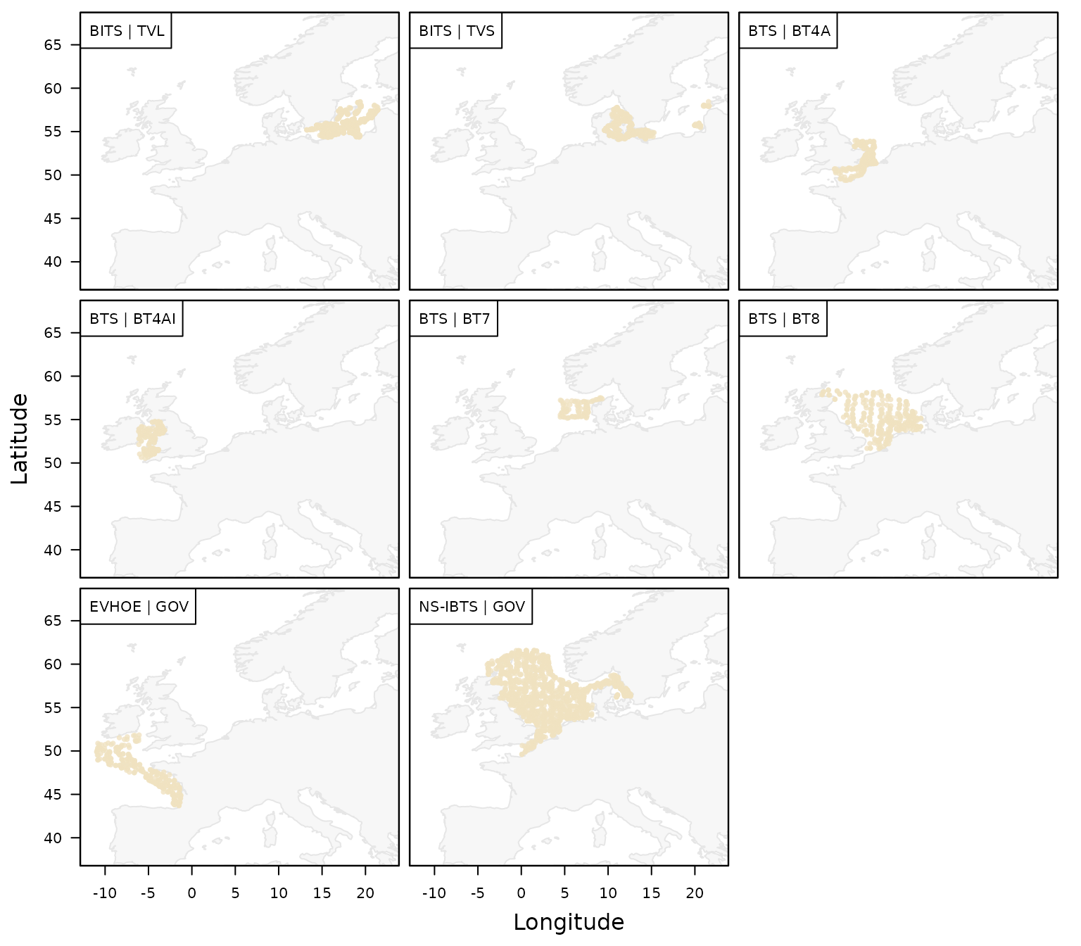

Points vs. gridded

By default, the function plots the actual haul locations, but it might be preferrable to aggregate the hauls and plot them by ICES statistical rectangle midpoints by setting the argument spatial_basis = "statrec":

plot_datras_overview(mini,
                     by_gear = TRUE,
                     spatial_basis = "statrec")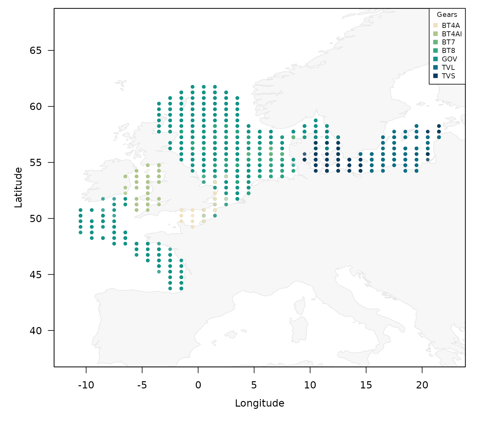

As multiple levels (here gears) might be present in a single ICES statistical rectangle, by default, the dominant level is assigned to that rectangle, but the argument grid_group_strategy allows to change that behaviour.

Instead of plots by statistical rectangle, the function also allows to plot an gridded image plot. This can be done by setting the mode = "grid":

plot_datras_overview(mini, by_gear = TRUE, mode = "grid")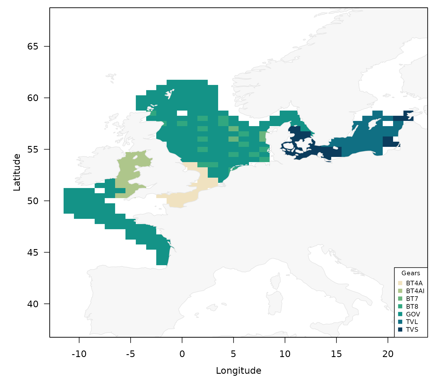

Again, by default the dominant level is shown for each grid cell.

Plotted quantity

While so far, the plots only quantified the absence / presence of a haul with a specific charactistics in each area, the function also allows us to plot various quantities by using the metric argument. We can for example plot the number of hauls with:

plot_datras_overview(mini,
                     mode = "grid",
                     metric = "count_hauls")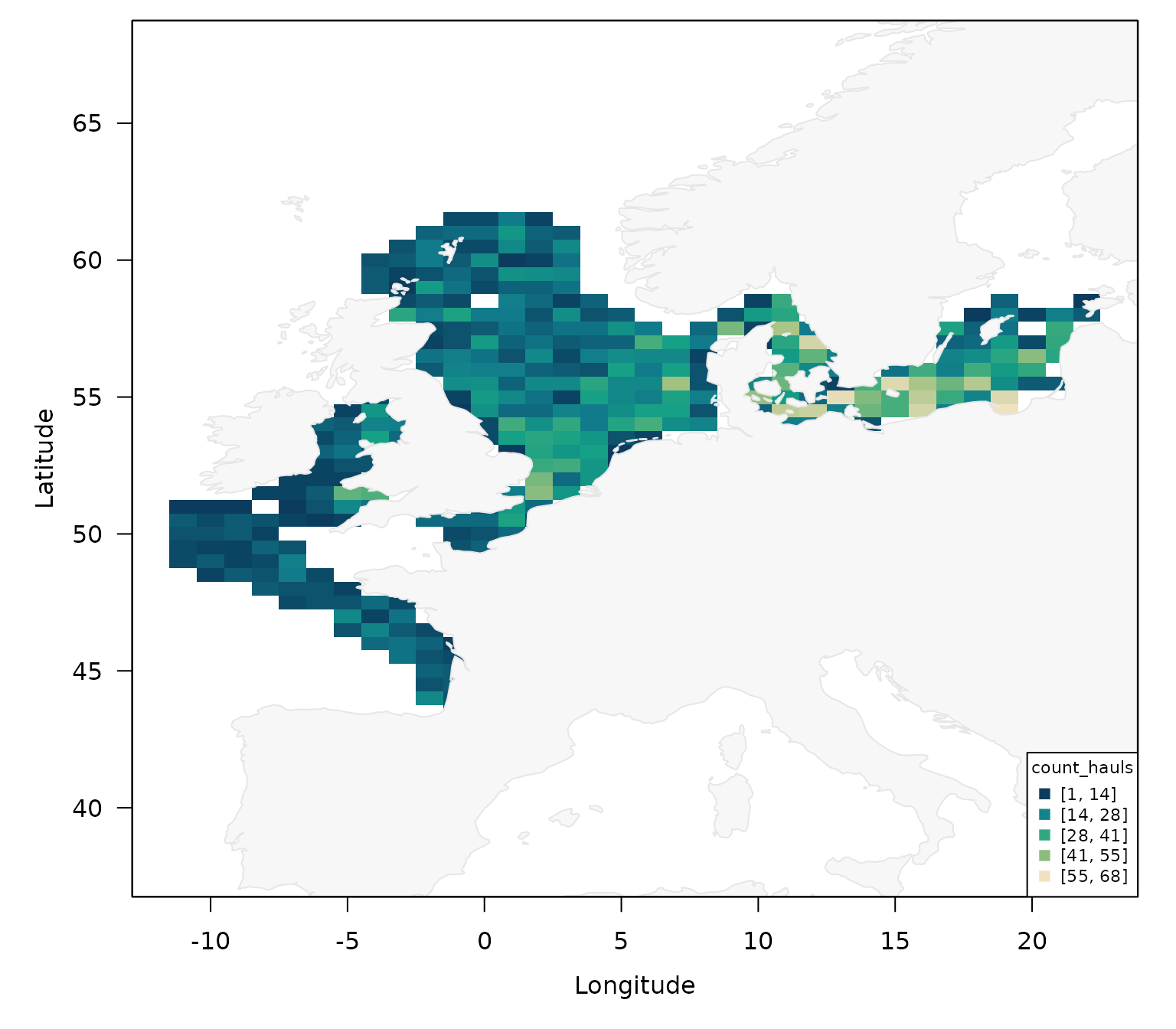

Note that this only works for the gridded mode and if requires the multi_panels = TRUE if you want to split it by another variable:

plot_datras_overview(mini,
                     mode = "grid",
                     metric = "count_hauls",
                     by_year = TRUE,
                     multi_panels = TRUE)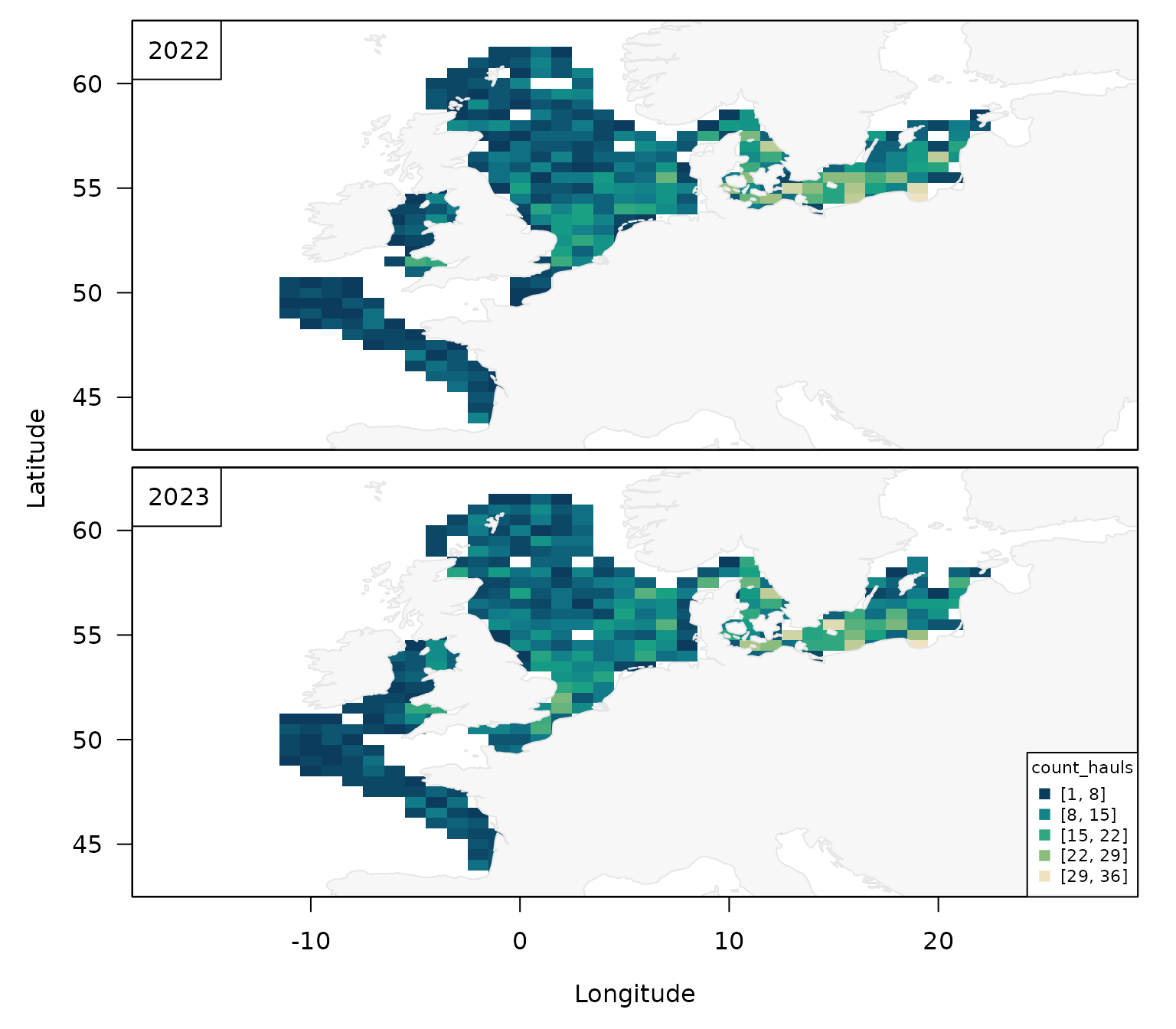

Similarly, you can plot the number of surveys by quarter:

plot_datras_overview(mini,
                     mode = "grid",
                     metric = "count_surveys",
                     by_quarter = TRUE,
                     multi_panels = TRUE)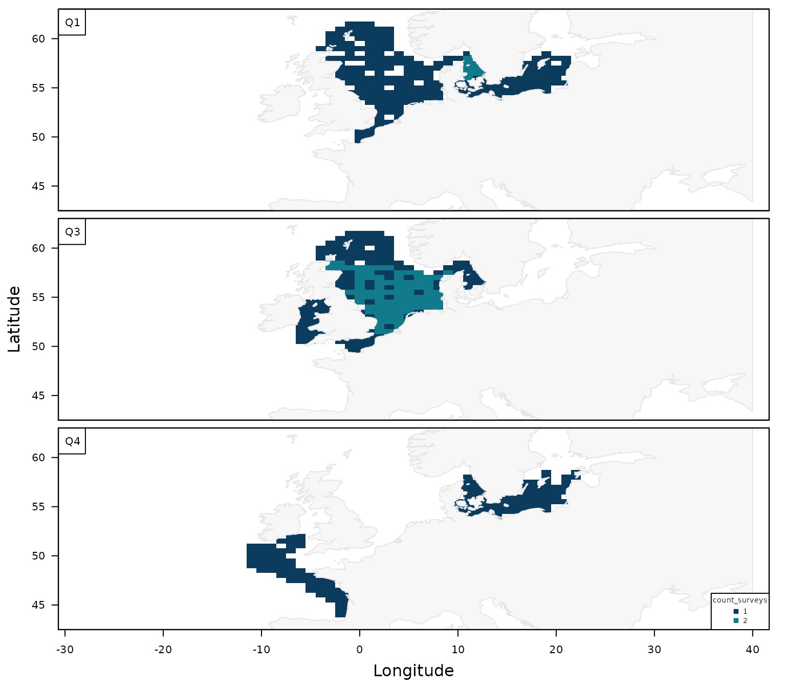

Other options of the metric argument are "sum" or "mean", but they become more meaningful when combined with the value_var argument (see below).

Value / Offset / Transform Workflows

If your DATRAS data set includes quantitative columns (for example a response and an effort-like offset), you can map transformed values in both grid and point modes. For example, a quick map of mean Depth can be created by:

plot_datras_overview(mini,
                     metric = "mean",
                     value_var = "Depth")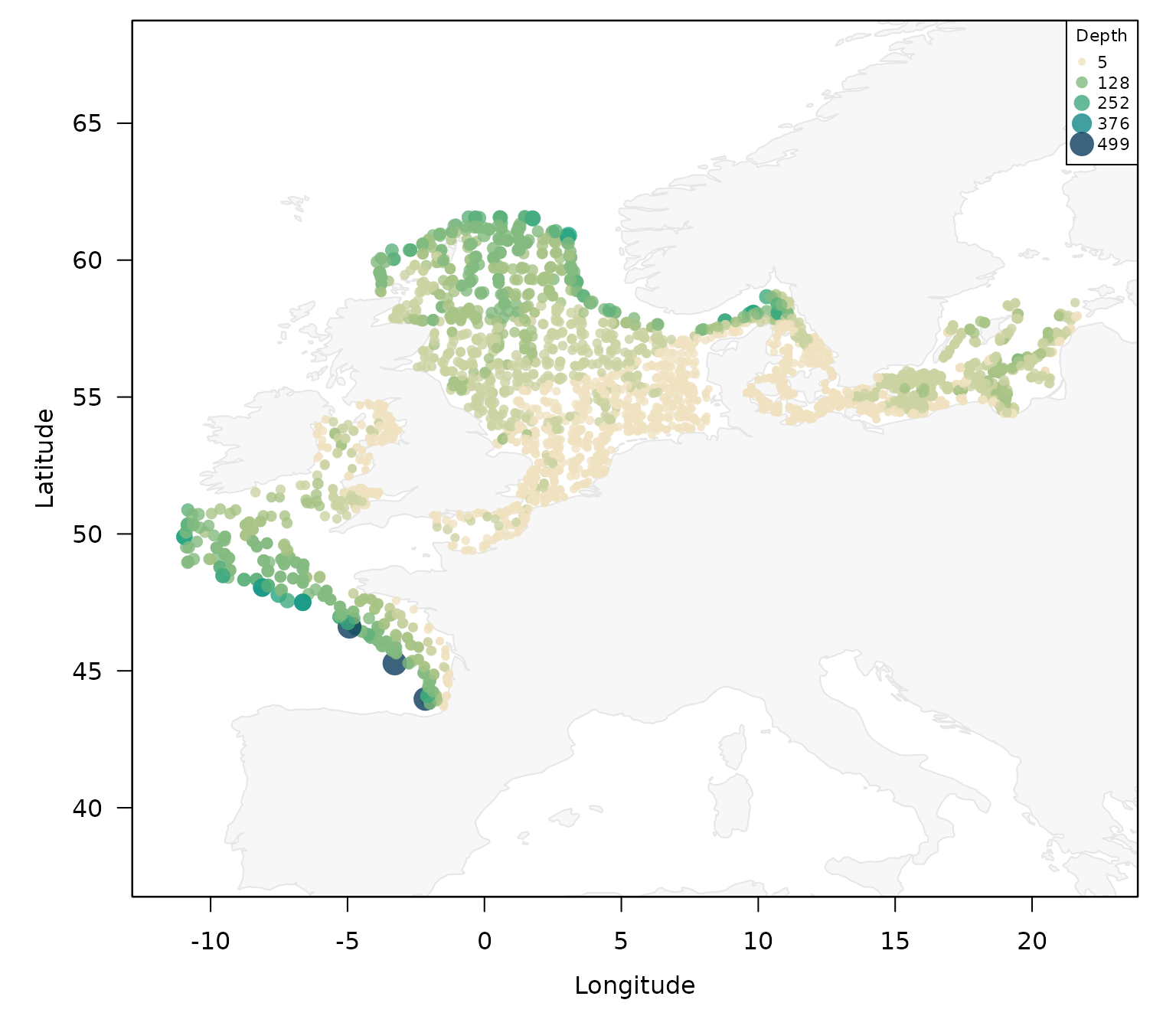

or as gridded version with squareroot transformation:

plot_datras_overview(mini,
                     mode = "grid",
                     metric = "mean",
                     value_var = "Depth",
                     transform = "sqrt")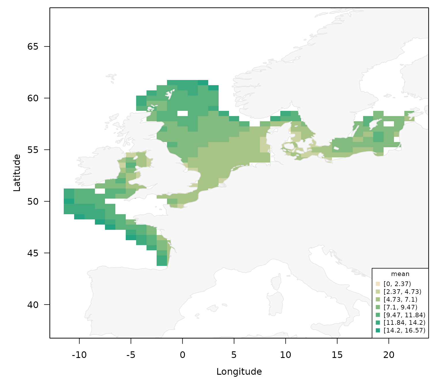

If your data set contains the number of individuals for example by using the DATRASextra workflow:

dab <- add_total_numbers_by_haul(dab)

Then the plotting function can be used to generate an overview of the hauls with the largest number of individuals:

plot_datras_overview(dab,
                     metric = "mean",
                     value_var = "HaulN")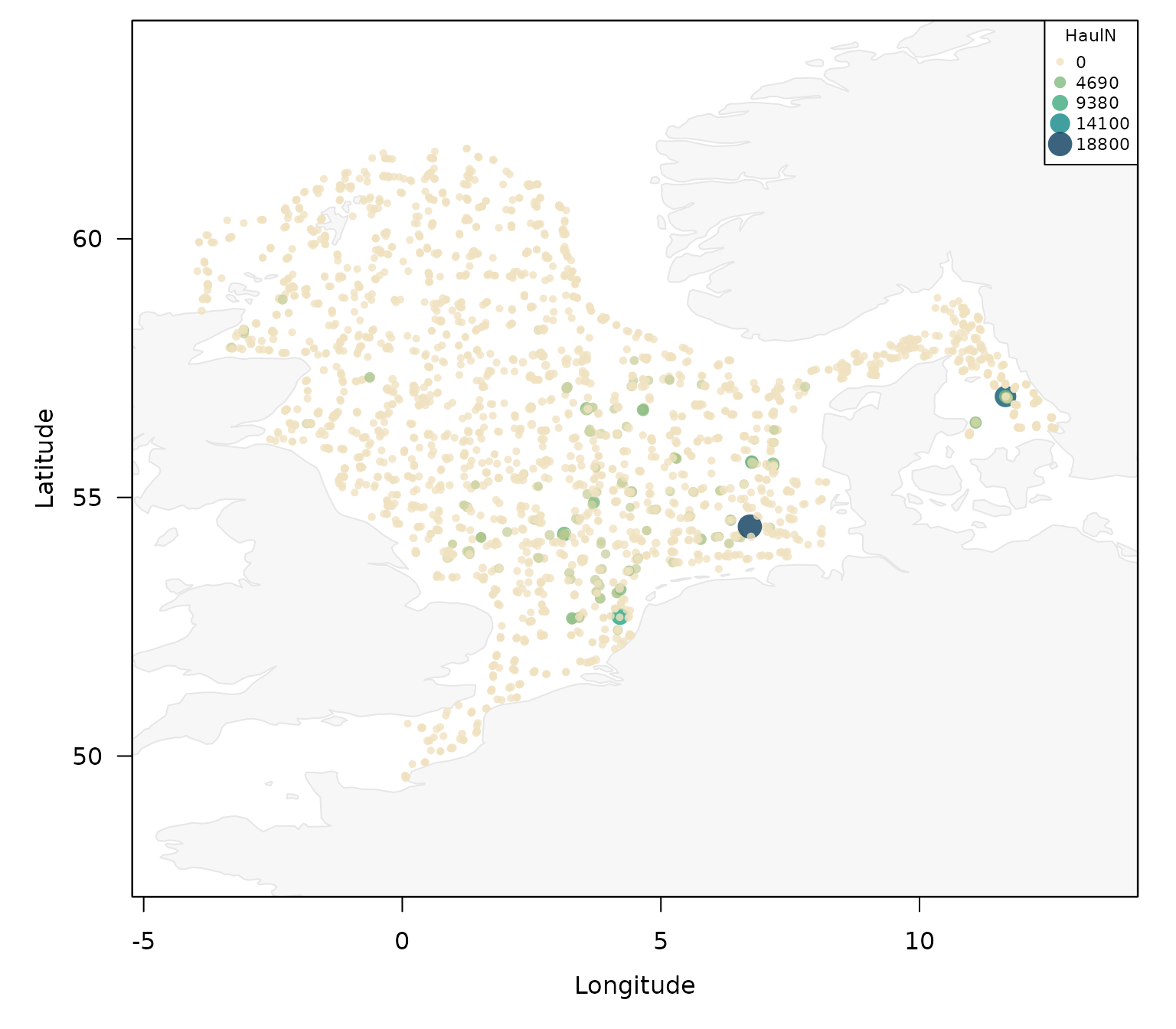

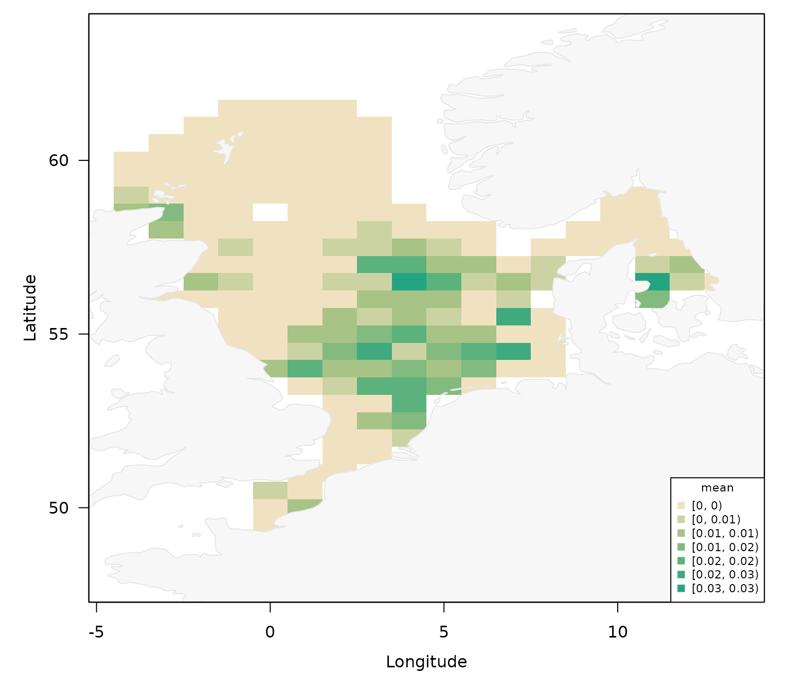
or as a gridded version:

plot_datras_overview(dab,
                     mode = "grid",
                     metric = "mean",
                     value_var = "HaulN")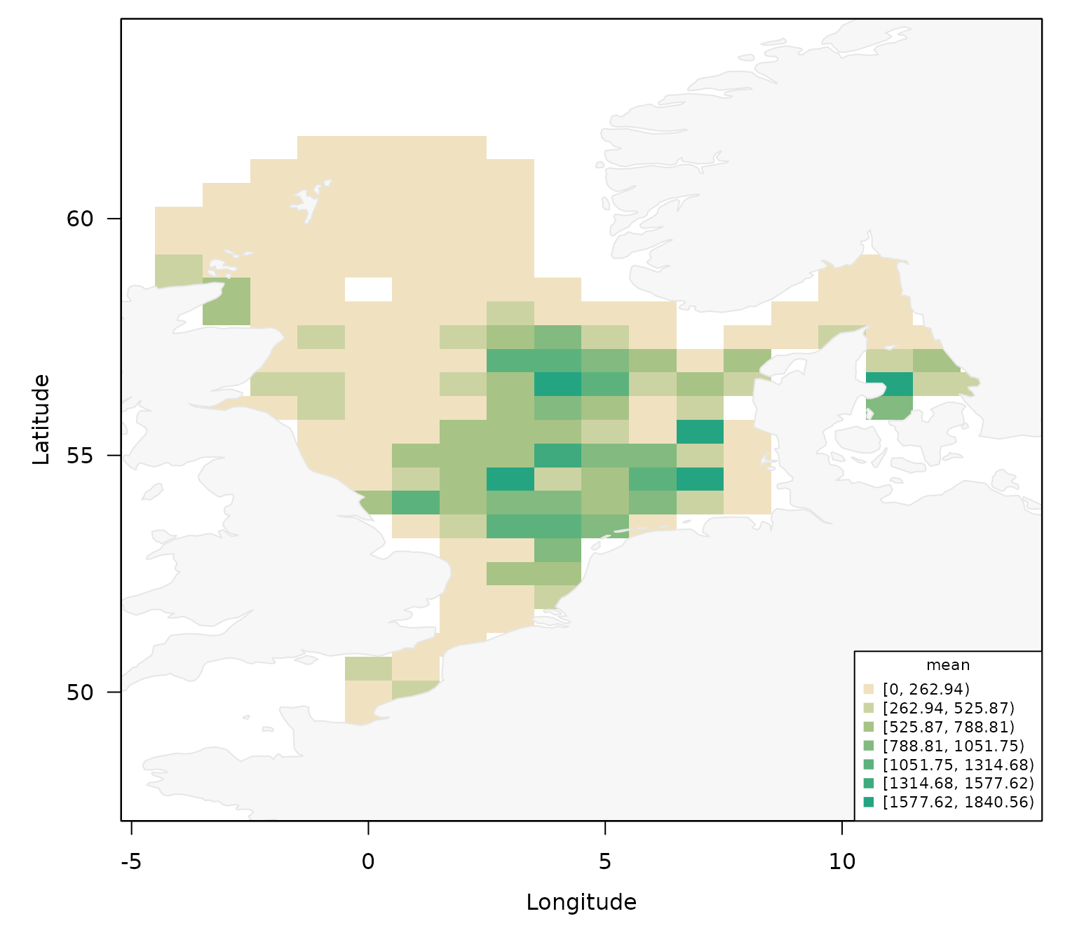

If in addition, a meaningful offset variable is available, such as haul duration or swept area for example by:

dab <- add_swept_area(dab)

Then this information can also be incorporated and the hauls with the largest numbers of individuals per offset can be plotted:

plot_datras_overview(dab,
                     metric = "mean",
                     value_var = "HaulN",
                     offset_var = "HaulDur")

or as a gridded version with swept area:

plot_datras_overview(dab,
                     mode = "grid",
                     metric = "mean",
                     value_var = "HaulN",
                     offset_var = "SweptArea")

Troubleshooting

If spatial_basis = "statrec" fails, check that StatRec exists and has valid values.
If no rows appear, verify xlim/ylim filters and coordinate columns.
If legends are suppressed in multi-panel mode, set legend_mode = "global".