
Building a spatiotemporal prediction grid
Source:vignettes/articles/make_spatiotemporal_grid.Rmd
make_spatiotemporal_grid.RmdThis article shows how to build a regular prediction grid over a
survey domain with make_survey_grid(), and how to extend it
into a spatiotemporal grid by repeating it across years. Such a
grid is a common input for spatial and spatiotemporal species
distribution models, where predictions are made on a regular lattice
covering the surveyed area.
We use the example data set dab (dab, Limanda
limanda, from the NS-IBTS
survey, 2020-2023).
## Load the packages
library(DATRASextra)
library(sf)

## Load the example data
data(dab)
Disclaimer
This is just one way of building a prediction grid. Choices such as the resolution, the distance threshold, and whether to remove land are subjective and should be tailored to your own data and objectives.
Trawl locations
We start from the unique haul positions in the HH table.
make_survey_grid() works directly on coordinate vectors, so
we only need the lon and lat columns.
## Unique trawl locations
trawls <- unique(dab[["HH"]][, c("haul.id", "lon", "lat")])
head(trawls)
#>                           haul.id    lon     lat
#> 1  NS-IBTS:2020:1:DK:26D4:GOV:6:1 7.1445 56.6076
#> 2  NS-IBTS:2020:1:DK:26D4:GOV:8:2 6.8874 56.5951
#> 3 NS-IBTS:2020:1:DK:26D4:GOV:10:3 7.1858 56.3057
#> 4 NS-IBTS:2020:1:DK:26D4:GOV:11:4 6.8544 56.3333
#> 5 NS-IBTS:2020:1:DK:26D4:GOV:19:5 2.4918 56.7180
#> 6 NS-IBTS:2020:1:DK:26D4:GOV:21:6 1.5045 56.7494
A spatial grid
make_survey_grid() builds an equally spaced grid
covering the range of the coordinates. resolution and
max_dist are expressed in the same units
as the coordinates — here degrees, because the hauls are in lon/lat. We
use a 0.1° grid and drop grid nodes that are more than 0.3° from any
haul, so the grid stays close to where the survey actually sampled (this
needs the RANN package).
## Regular grid near the trawl observations
grid <- make_survey_grid(
  x          = trawls$lon,
  y          = trawls$lat,
  resolution = 0.1,
  max_dist   = 0.3
)

nrow(grid)
#> [1] 8326
head(grid)
#>      X    Y
#> 1 -0.2 49.5
#> 2 -0.1 49.5
#> 3  0.0 49.5
#> 4  0.1 49.5
#> 5  0.2 49.5
#> 6  0.3 49.5
The result is a data frame with columns X and
Y. A quick plot shows the grid following the survey
footprint:
## Grid nodes (blue) and trawl observations (red)
plot(grid$X, grid$Y, pch = 15, col = "lightblue", cex = 0.5,
     xlab = "Longitude", ylab = "Latitude")
points(trawls$lon, trawls$lat, col = "red", pch = 20, cex = 0.6)
legend("topright", legend = c("Prediction grid", "Trawl observations"),
       col = c("lightblue", "red"), pch = c(15, 20), bg = "white")
box(lwd = 1.5)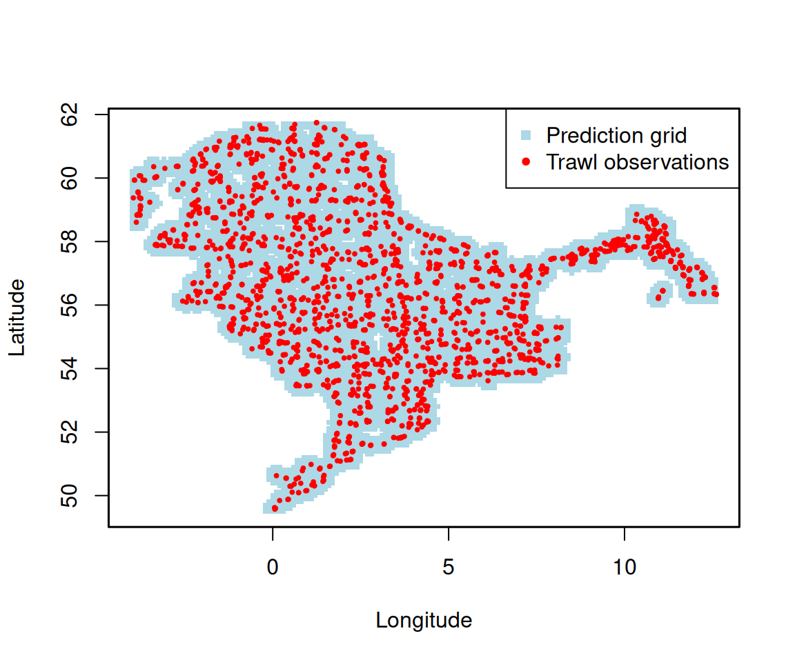
For predictions in true distance units, project the coordinates first
(for example to UTM), pass the projected coordinates to
make_survey_grid(), and set resolution and
max_dist in metres or kilometres.
Adding the time dimension
To turn the spatial grid into a spatiotemporal one, pass a
vector of years to time. The spatial grid is then repeated
for each year and a year column is added, giving one row
per grid node and year.
## Repeat the grid across survey years
grid_st <- make_survey_grid(
  x          = trawls$lon,
  y          = trawls$lat,
  resolution = 0.1,
  max_dist   = 0.2,
  time       = 2020:2023
)

nrow(grid_st)
#> [1] 27424
head(grid_st)
#>      X    Y year
#> 1 -0.1 49.5 2020
#> 2  0.0 49.5 2020
#> 3  0.1 49.5 2020
#> 4  0.2 49.5 2020
#> 5 -0.1 49.6 2020
#> 6  0.0 49.6 2020
## One spatial grid per year
table(grid_st$year)
#>
#> 2020 2021 2022 2023
#> 6856 6856 6856 6856
This grid_st data frame - with X,
Y, and year - can be passed directly to a
spatiotemporal model as the set of locations to predict on.
Projected coordinates
Distances in degrees are not equal in all directions: in the North
Sea a degree of longitude is only about 60 % of a degree of latitude.
For a grid in kilometres, project the haul positions first.
add_xy() adds the columns X and Y
(by default the European equal-area projection EPSG:3035, in km) to
HH, and with inverse = TRUE adds longitude and
latitude to a projected grid.
## Haul positions in km
dab_xy <- add_xy(dab)
hauls <- unique(dab_xy[["HH"]][, c("haul.id", "X", "Y", "Year", "Quarter", "Depth")])
hauls$Year <- as.numeric(as.character(hauls$Year))

## 10 km grid, nodes within 15 km of a haul
grid_km <- make_survey_grid(hauls$X, hauls$Y, resolution = 10, max_dist = 15)

## Longitude and latitude of each node
grid_km <- add_xy(grid_km, inverse = TRUE)
head(grid_km)
#>      X    Y          lon      lat
#> 1 3600 2980  0.014874692 49.49112
#> 2 3610 2980  0.151863840 49.50323
#> 3 3590 2990 -0.140748963 49.56780
#> 4 3600 2990 -0.003577597 49.58010
#> 5 3610 2990  0.133656846 49.59223
#> 6 3620 2990  0.270953566 49.60419
Filling gaps
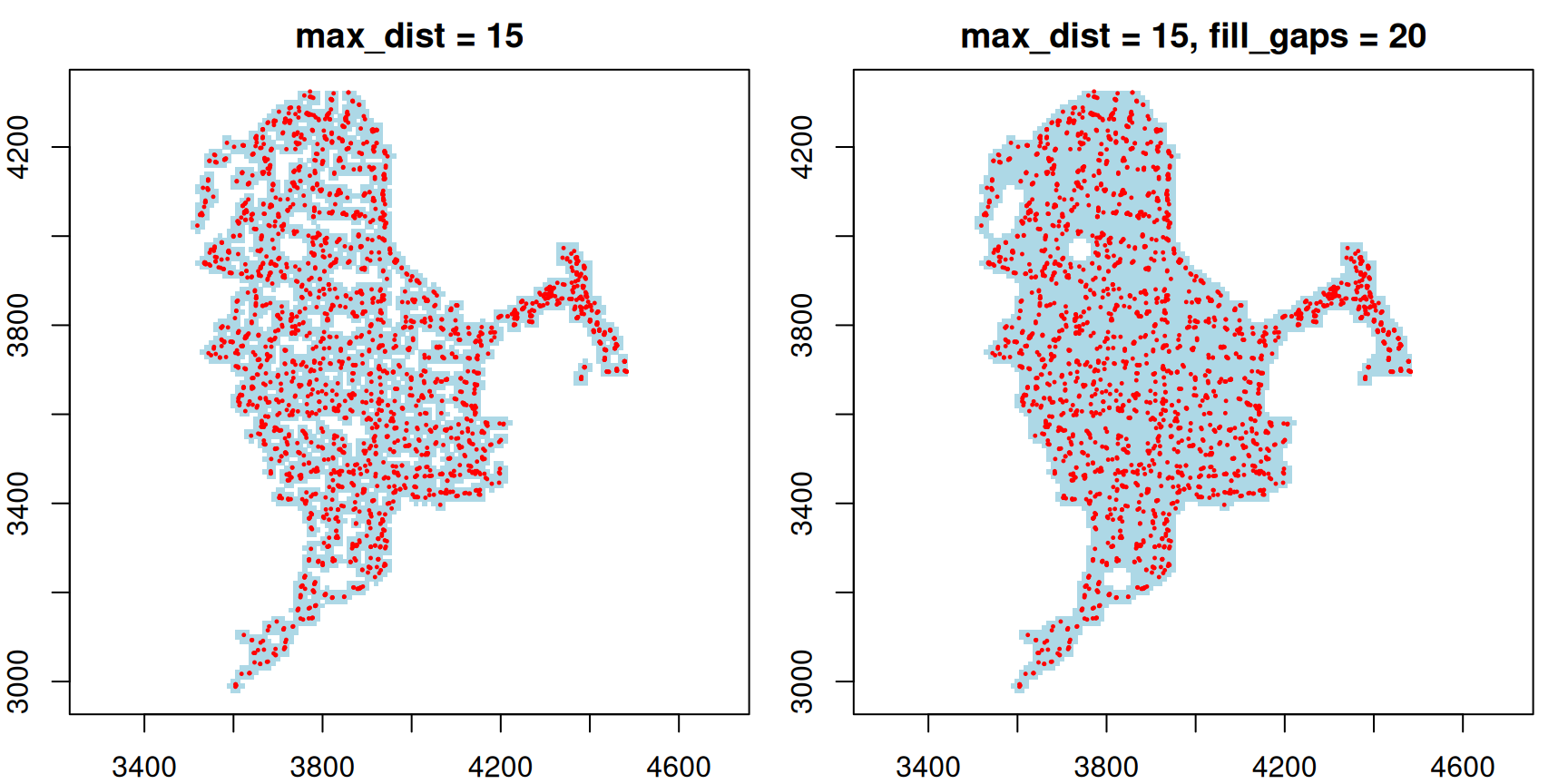
With max_dist alone, a grid node is kept only when a
haul lies within max_dist. Where the hauls are farther
apart than 2 * max_dist, this leaves holes inside the
survey area and notches along its edge, although the survey covers the
area between them. A larger max_dist would close the holes,
but would also push the outer edge further from the outermost hauls.
fill_gaps closes holes and bays narrower than about
2 * fill_gaps and leaves the outer edge where
max_dist put it. The footprint is first grown by
max_dist + fill_gaps around each haul, then shrunk by
fill_gaps again.
grid_filled <- make_survey_grid(hauls$X, hauls$Y, resolution = 10,
                                max_dist = 15, fill_gaps = 20)
c(without = nrow(grid_km), with = nrow(grid_filled))
#> without    with
#>    4357    5235

grids <- list("max_dist = 15" = grid_km,
              "max_dist = 15, fill_gaps = 20" = grid_filled)
par(mfrow = c(1, 2), mar = c(2, 2, 2, 1))
for (nm in names(grids)) {
  g <- grids[[nm]]
  plot(g$X, g$Y, pch = 15, cex = 0.4, col = "lightblue", asp = 1,
       xlab = "", ylab = "", main = nm)
  points(hauls$X, hauls$Y, pch = 20, cex = 0.3, col = "red")
}
Where the survey sampled each year
A spatiotemporal model predicts into every node in every year, also
in years in which no haul came near a node.
add_grid_support() flags this. It adds
supported, which is TRUE when the hauls of a
year, or of the years at most window away, cover the node,
and coverage, the share of years in which a node is
covered. Coverage is checked with the same max_dist and
fill_gaps as the grid.
Surveys often cover different areas in different quarters, so the grid is built per quarter, here for quarter 1.
years <- sort(unique(hauls$Year))
q1 <- hauls[hauls$Quarter == "1", ]

grid_q1 <- make_survey_grid(hauls$X, hauls$Y, resolution = 10, max_dist = 15,
                            fill_gaps = 20, time = years)
grid_q1 <- add_grid_support(grid_q1, q1$X, q1$Y, q1$Year,
                            max_dist = 15, fill_gaps = 20, window = 1)

## Keep the nodes covered in at least a quarter of the years
grid_q1 <- grid_q1[grid_q1$coverage >= 0.25, ]

## Share of supported nodes per year
tapply(grid_q1$supported, grid_q1$year, mean)
#>      2020      2021      2022      2023
#> 0.9677959 0.9797156 0.9454203 0.8322877
Predictions for unsupported nodes are extrapolations. They can be dropped, or kept and marked on the maps.
Adding depth
Depth is a common covariate in distribution models, and a check that
the grid stays within the depths the survey fishes.
add_bathymetry() adds the depth from NOAA’s ETOPO
bathymetry (through the marmap package). With
path, the download is kept and reused.
depth_range adds depth_ok, whether a node lies
within a depth range, here that of 98 % of the hauls.
Removing land (optional)
A rectangular grid can include cells that fall on land. If your model domain is sea only, drop those cells. Here we use coastline polygons from Natural Earth and keep only grid nodes that fall in the sea.
library(rnaturalearth)

## Land polygon (WGS84)
land <- st_union(st_make_valid(ne_countries(scale = 10, returnclass = "sf")))

## Keep only grid nodes that are not on land
grid_sf <- st_as_sf(grid, coords = c("X", "Y"), crs = 4326)
on_land <- lengths(st_intersects(grid_sf, land)) > 0
grid_sea <- grid[!on_land, ]
Cross grid_sea with the survey years (as above) to
obtain a sea-only spatiotemporal grid.