Deriving numbers and weight by haul and custom length classes

This vignette demonstrates how to derive numbers and weight by haul from ICES DATRAS survey data using DATRASextra. It shows how to

create a haul-by-length matrix of numbers,
convert numbers at length to weight at length,
aggregate these quantities over custom length classes, and
derive haul-level summaries for all fish combined or for user-defined length groups such as juveniles and adults.

These summaries are useful for survey standardisation, indicator development, biodiversity analyses, and stock-assessment workflows.

Outline

Load DATRASextra
Create numbers at length
Convert numbers at length to weight at length
Aggregate numbers and weight over custom length classes
Summary
References

Load DATRASextra

Load the package with:

library(DATRASextra)

This vignette assumes that a cleaned DATRAS data set is already available. For a full workflow covering download, reading, and cleaning of survey data, see vignette("datrasextra-tutorial").

Here, we use the example data set dab included in the package and apply a standard cleaning step first:

dab <- clean_datras(dab)

Create numbers at length

Catch-at-length information is stored in the HL component of a DATRAS object. Before aggregating these data, it is useful to inspect the available length measurements:

lpars <- check_lengths(dab)
#> [1] "Length statistics:"
#>          min  mean median maxObs maxEmp perc
#> 99.9999%   3 17.36   17.5     43     40 37.5
#> [1] "Observations above:"
#>         maxLEmp percL
#> Numbers   1e+00 1e+00
#> Percent   1e-04 1e-04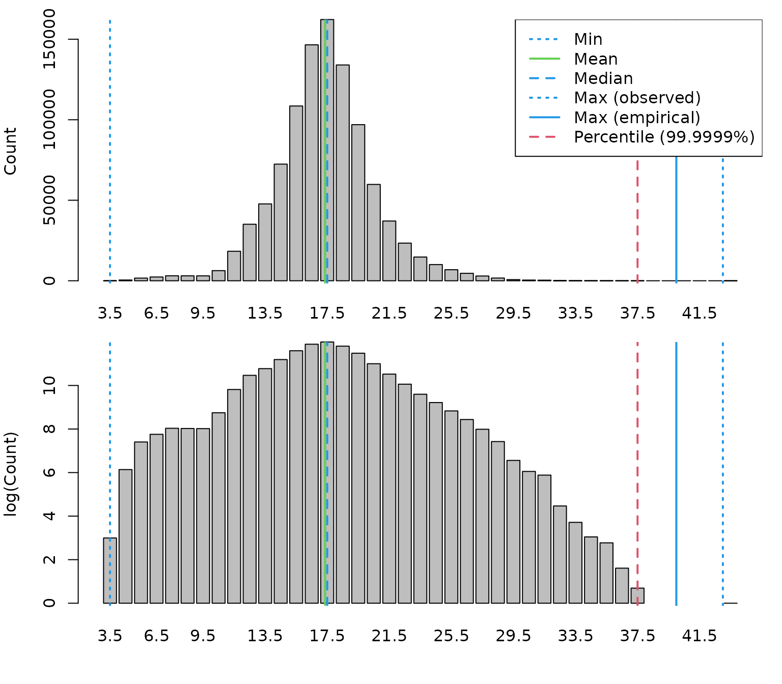

This function provides summary statistics and diagnostic plots of the recorded lengths. It can help identify potential data issues such as implausible values or unusual length distributions. If the data look reasonable, the next step is to aggregate the HL observations to numbers at length by haul and add the result to the HH component:

dab <- add_numbers_at_length(dab)

This creates a matrix HH$N, with one row per haul and one column per length class:

dab[["HH"]][["N"]][1:5, 1:5]
#>                                      sizeGroup
#> haul.id                               [3,4) [4,5) [5,6) [6,7) [7,8)
#>   NS-IBTS:2020:1:NO:58G2:GOV:60055:55     0     0     0     0     0
#>   NS-IBTS:2020:1:NO:58G2:GOV:60054:54     0     0     0     0     0
#>   NS-IBTS:2020:1:NO:58G2:GOV:60053:53     0     0     0     0     0
#>   NS-IBTS:2020:1:NO:58G2:GOV:60052:52     0     0     0     0     0
#>   NS-IBTS:2020:1:NO:58G2:GOV:60051:51     0     0     0     0     0

By default, add_numbers_at_length() defines length classes from the minimum and maximum observed lengths, using the coarsest length recording resolution present in the data (see ?get_accuracy_cm). In most cases, this is a sensible default.

If a different resolution or range is needed, custom breaks can be supplied via cm_breaks and by. In general, it is recommended to keep the numbers-at- length matrix as fine as possible, because these length classes are also used to derive weights at length in the next step. Coarser groupings can then be obtained later with add_total_numbers_by_haul() or add_total_weight_by_haul().

For example, the following code creates numbers at length using 0.5 cm bins:

## Define custom resolution of length bins
by <- 0.5

## Define custom length bins
cm_breaks <- seq(lpars$lPars$min, lpars$lPars$maxEmp, by = by)

## Recalculate numbers at length using custom bins
dab <- add_numbers_at_length(dab, cm_breaks = cm_breaks, by = by)

The resulting matrix now has a finer length resolution:

dab[["HH"]][["N"]][1:5, 1:5]
#>                                      sizeGroup
#> haul.id                               [3,3.5) [3.5,4) [4,4.5) [4.5,5) [5,5.5)
#>   NS-IBTS:2020:1:NO:58G2:GOV:60055:55       0       0       0       0       0
#>   NS-IBTS:2020:1:NO:58G2:GOV:60054:54       0       0       0       0       0
#>   NS-IBTS:2020:1:NO:58G2:GOV:60053:53       0       0       0       0       0
#>   NS-IBTS:2020:1:NO:58G2:GOV:60052:52       0       0       0       0       0
#>   NS-IBTS:2020:1:NO:58G2:GOV:60051:51       0       0       0       0       0

Convert numbers at length to weight at length

Numbers at length are sufficient for some applications, but many analyses also require biomass or weight by length class or by haul. For example, biomass-based survey indices are often used in stock assessment or ecosystem analyses.

To derive weights, DATRASextra uses the individual length and weight records stored in the CA component to estimate a length-weight relationship. Before doing so, it is useful to inspect the available weight data:

wpars <- check_weights(dab)
#> [1] "Length statistics:"
#>   min  mean median max
#> 1   3 18.94     19  35
#> [1] "Weight statistics:"
#>   min  mean median max
#> 1   1 85.93     66 559
#> [1] "Estimated LW parameters:"
#> [1] "a = 0.014 b = 2.903"
#> [1] "Lookup LW parameters in the species_info table:"
#> [1] "a = 0.007 b = 3.119"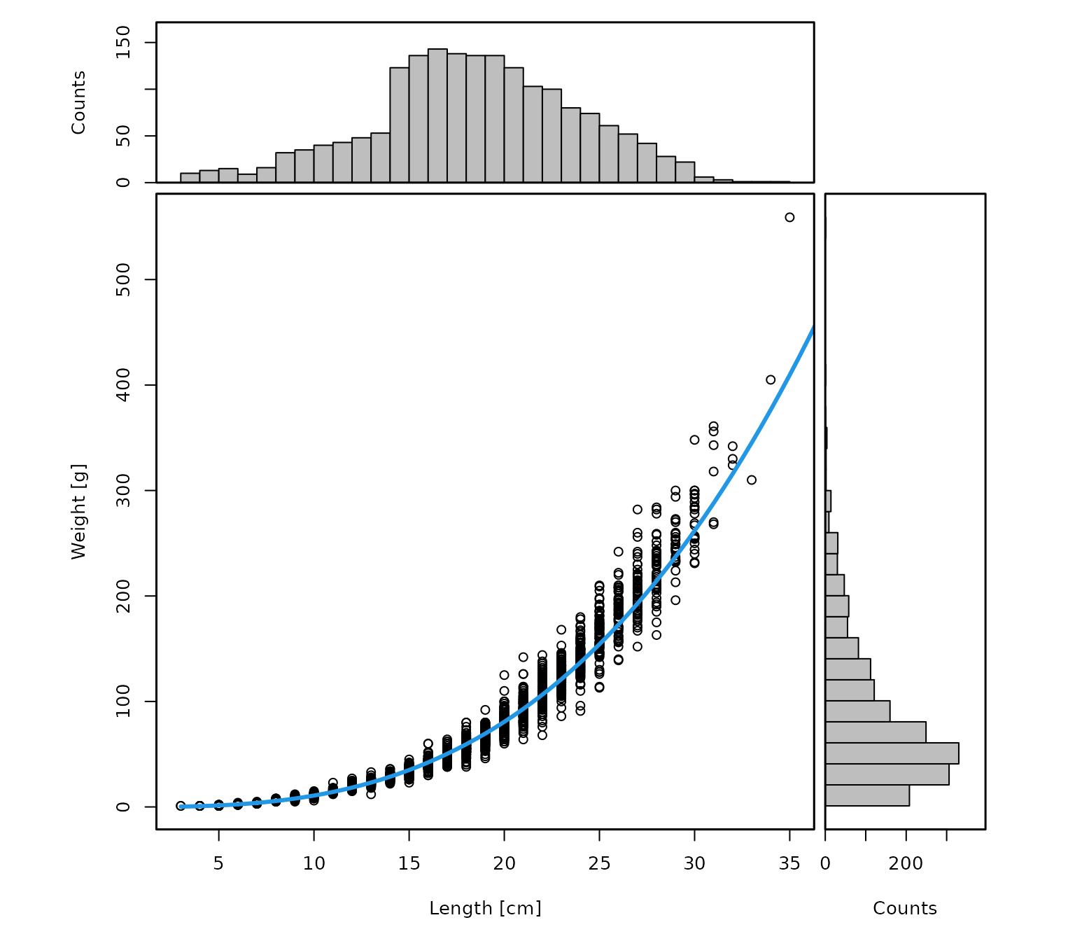

This function provides summary statistics and diagnostic plots for the weight data and the fitted length-weight relationship. If the information looks reasonable, the numbers-at-length matrix in HH$N can be converted to weight at length with:

dab <- add_weight_at_length(dab)

This adds a matrix HH$Wgt, containing the estimated weight in each length class for each haul.

The function uses the midpoints of the existing length bins in HH$N (stored in attr(dab, "cm.breaks")) and converts these lengths to weights using the fitted length-weight relationship from the CA data.

One important caveat concerns the largest length class. If the final bin is a plus group with a very large upper limit, such as Inf, or extends far beyond the observed size range, the midpoint of that bin may imply an unrealistically large weight. In such cases, it may be preferable to use the plus_group argument.

If the CA component does not contain enough information to estimate a reliable length-weight relationship, lookup parameters can instead be taken from the species_info table by setting lw_source = "lookup". Before doing so, it is good practice to inspect the stored parameters:

species_info[
  which(species_info$ScientificName_WoRMS == "Limanda limanda"),
  c("a", "b")
]
#>          a     b
#> 1017 0.007 3.119

If these values appear appropriate, the lookup relationship in the species_info table can be used with:

dab <- add_weight_at_length(dab, lw_source = "lookup")

Aggregate numbers and weight over custom length classes

By default, add_total_numbers_by_haul() and add_total_weight_by_haul() sum over all available length classes and return one total value per haul. In many applications, however, it is useful to retain separate haul-level summaries for custom length groups, for example juveniles and adults.

For dab, one biologically meaningful split is the approximate length at 50% maturity, available in species_info:

(lm <- species_info[
  which(species_info$ScientificName_WoRMS == "Limanda limanda"),
  "Lm"
])
#> [1] 17.75

We can use this value to define two custom groups, below and above Lm:

length_cuts <- c(0, lm, Inf)

dab <- add_total_numbers_by_haul(dab, length_cuts = length_cuts)
dab <- add_total_weight_by_haul(dab, length_cuts = length_cuts)

This returns haul-level summaries for juveniles and adults separately:

head(dab[["HH"]][["HaulN"]])
#>                                     (0-17.75] (17.75-Inf]
#> NS-IBTS:2020:1:NO:58G2:GOV:60055:55         0           0
#> NS-IBTS:2020:1:NO:58G2:GOV:60054:54         0           0
#> NS-IBTS:2020:1:NO:58G2:GOV:60053:53        82         221
#> NS-IBTS:2020:1:NO:58G2:GOV:60052:52       523         543
#> NS-IBTS:2020:1:NO:58G2:GOV:60051:51        42         144
#> NS-IBTS:2020:1:NO:58G2:GOV:60050:50         0           0

head(dab[["HH"]][["HaulWgt"]])
#>                                     (0-17.75] (17.75-Inf]
#> NS-IBTS:2020:1:NO:58G2:GOV:60055:55     0.000        0.00
#> NS-IBTS:2020:1:NO:58G2:GOV:60054:54     0.000        0.00
#> NS-IBTS:2020:1:NO:58G2:GOV:60053:53  4256.383    25914.94
#> NS-IBTS:2020:1:NO:58G2:GOV:60052:52 24487.167    48769.12
#> NS-IBTS:2020:1:NO:58G2:GOV:60051:51  1989.542    15829.06
#> NS-IBTS:2020:1:NO:58G2:GOV:60050:50     0.000        0.00

By default, the column names reflect the chosen cut points, but they can be renamed as needed:

colnames(dab[["HH"]][["HaulN"]]) <- c("juveniles", "adults")
colnames(dab[["HH"]][["HaulWgt"]]) <- c("juveniles", "adults")

This makes the result easier to interpret:

head(dab[["HH"]][["HaulN"]])
#>                                     juveniles adults
#> NS-IBTS:2020:1:NO:58G2:GOV:60055:55         0      0
#> NS-IBTS:2020:1:NO:58G2:GOV:60054:54         0      0
#> NS-IBTS:2020:1:NO:58G2:GOV:60053:53        82    221
#> NS-IBTS:2020:1:NO:58G2:GOV:60052:52       523    543
#> NS-IBTS:2020:1:NO:58G2:GOV:60051:51        42    144
#> NS-IBTS:2020:1:NO:58G2:GOV:60050:50         0      0

Of course, any number of custom length groups can be defined. For example:

length_cuts <- c(0, 10, 20, 30, 100)

dab <- add_total_numbers_by_haul(dab, length_cuts = length_cuts)
dab <- add_total_weight_by_haul(dab, length_cuts = length_cuts)

This gives haul-level numbers and weights for four user-defined length groups:

head(dab[["HH"]][["HaulN"]])
#>                                     (0-10] (10-20] (20-30] (30-100]
#> NS-IBTS:2020:1:NO:58G2:GOV:60055:55      0       0       0        0
#> NS-IBTS:2020:1:NO:58G2:GOV:60054:54      0       0       0        0
#> NS-IBTS:2020:1:NO:58G2:GOV:60053:53      0     186     105       12
#> NS-IBTS:2020:1:NO:58G2:GOV:60052:52      0     853     213        0
#> NS-IBTS:2020:1:NO:58G2:GOV:60051:51      0      99      85        2
#> NS-IBTS:2020:1:NO:58G2:GOV:60050:50      0       0       0        0
head(dab[["HH"]][["HaulWgt"]])
#>                                     (0-10]   (10-20]  (20-30] (30-100]
#> NS-IBTS:2020:1:NO:58G2:GOV:60055:55      0     0.000     0.00    0.000
#> NS-IBTS:2020:1:NO:58G2:GOV:60054:54      0     0.000     0.00    0.000
#> NS-IBTS:2020:1:NO:58G2:GOV:60053:53      0 11691.009 14499.36 3980.953
#> NS-IBTS:2020:1:NO:58G2:GOV:60052:52      0 48278.947 24977.34    0.000
#> NS-IBTS:2020:1:NO:58G2:GOV:60051:51      0  6120.161 10719.41  979.030
#> NS-IBTS:2020:1:NO:58G2:GOV:60050:50      0     0.000     0.00    0.000

These summaries can then be used to explore whether the spatial distribution differs among size groups. For example, the following plot shows where hauls with positive catches occurred for each length class, with point size scaled by haul-level abundance:

ncols <- ncol(dab[["HH"]][["HaulWgt"]])

par(mfrow = n2mfrow(ncols, asp = 2),
    mar = c(3, 3, 2, 2),
    oma = c(2, 2, 0, 0))

for (i in seq_len(ncols)) {
  plot(dab[["HH"]]$lon, dab[["HH"]]$lat,
       type = "n",
       xlab = "", ylab = "",
       main = colnames(dab[["HH"]]$HaulN)[i])

  ind <- which(dab[["HH"]]$HaulN[, i] > 0)

  points(dab[["HH"]]$lon[ind], dab[["HH"]]$lat[ind],
         cex = dab[["HH"]]$HaulN[, i][ind] /
           max(dab[["HH"]]$HaulN[, i][ind]) * 3,
         col = i)
}

mtext("Longitude", 1, outer = TRUE)
mtext("Latitude", 2, outer = TRUE)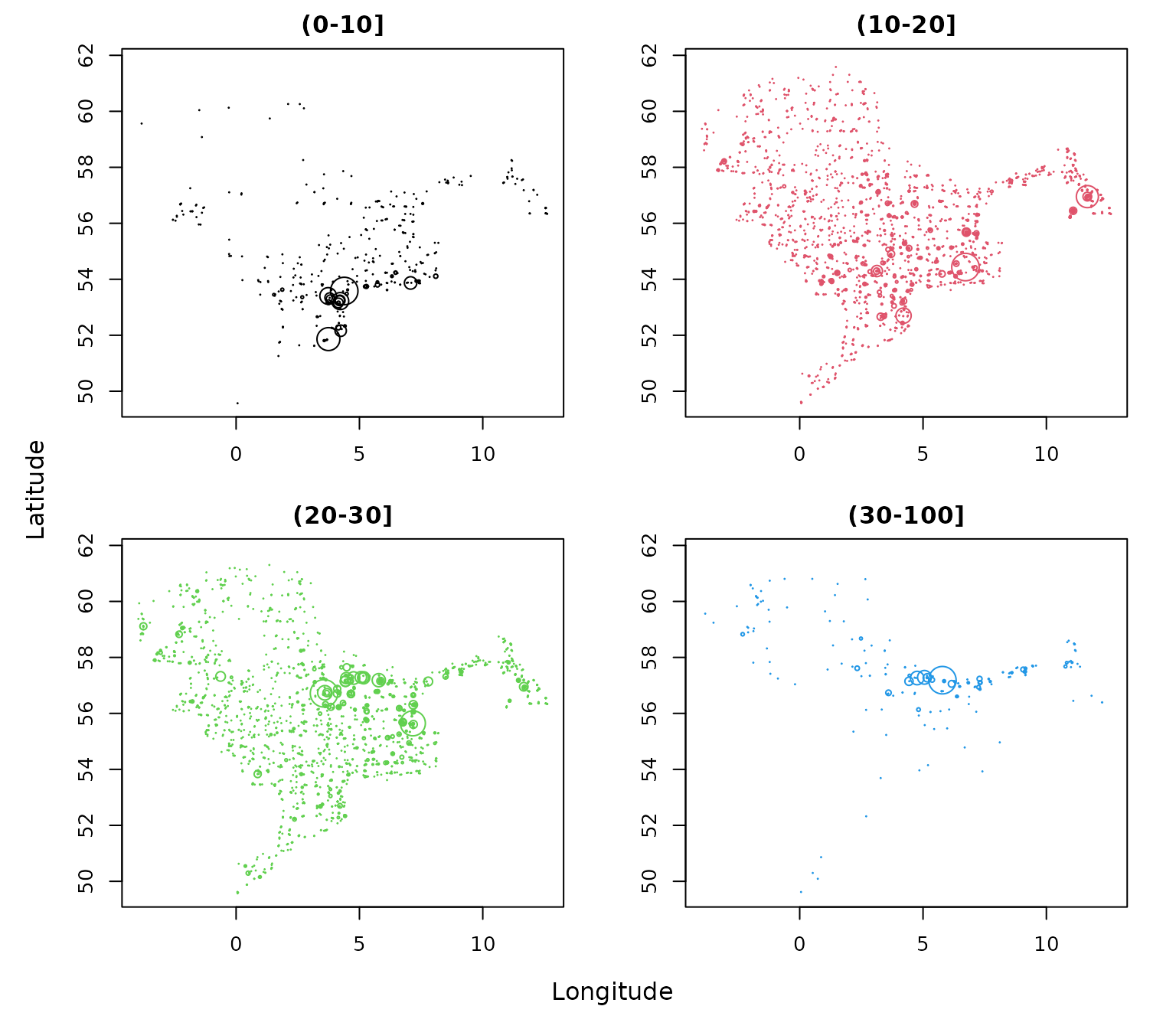

Summary

This vignette showed how to derive haul-level abundance and biomass summaries from DATRAS data using DATRASextra. Starting from a cleaned survey data set, it demonstrated how to inspect the available length and weight information, construct a numbers-at-length matrix, convert numbers at length to weight at length, and aggregate both quantities over custom length classes.